TP - Partie 3

Pour aller plus loin

Author

C.Maugis-Rabusseau et V.Rocher

Published

June 6, 2025

library(Seurat)
library(SeuratData)
library(BayesSpace)
library(ggplot2)
source("Cours/FunctionsAux.R")

1 Spatial transcriptomic (ST)

1.1 Données de l’exemple

Description:

Données de transcirptomique spatiale du cerveau de la souris pour la région antérieure
Expression de \(G=31053\) gènes pour \(C=2696\) spots

InstallData("stxBrain")

Warning: The following packages are already installed and will not be
reinstalled: stxBrain

brain <- LoadData("stxBrain", type = "anterior1")

Validating object structure

Updating object slots

Ensuring keys are in the proper structure
Ensuring keys are in the proper structure

Ensuring feature names don't have underscores or pipes

Updating slots in Spatial

Updating slots in anterior1

Validating object structure for Assay5 'Spatial'

Validating object structure for VisiumV2 'anterior1'

Object representation is consistent with the most current Seurat version

brain

An object of class Seurat 
31053 features across 2696 samples within 1 assay 
Active assay: Spatial (31053 features, 0 variable features)
 1 layer present: counts
 1 spatial field of view present: anterior1

brain@assays$Spatial$counts[1:6,1:10]

6 x 10 sparse Matrix of class "dgCMatrix"

  [[ suppressing 10 column names 'AAACAAGTATCTCCCA-1', 'AAACACCAATAACTGC-1', 'AAACAGAGCGACTCCT-1' ... ]]

                           
Xkr4    . . . . . . . . . .
Gm1992  . . . . . . . . . .
Gm37381 . . . . . . . . . .
Rp1     . . . . . . . . . .
Sox17   . 1 . . . 2 . . 1 .
Gm37323 . . . . . . . . . .

brain@images$anterior1

Spatial coordinates for 2696 cells
Default segmentation boundary: centroids 
Associated assay: Spatial 
Key: slice1_

SpatialFeaturePlot(brain, features = "nCount_Spatial") + 
  theme(legend.position = "right")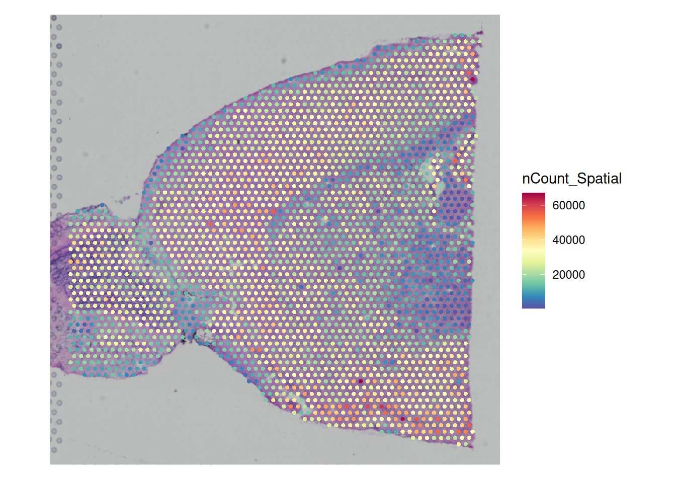

1.2 Normalisation avec SCTransform

Comprend les étapes de normalisation, calcul des HVG et scale data

brain <- SCTransform(brain, assay = "Spatial", verbose = FALSE)
brain@assays$SCT

SCTAssay data with 17668 features for 2696 cells, and 1 SCTModel(s) 
Top 10 variable features:
 Ttr, Hbb-bs, Mbp, Plp1, Hba-a1, Ptgds, Penk, S100a5, Hba-a2, Fabp7

plot1<-VariableFeaturePlot(brain)
top10<-head(VariableFeatures(brain), 10)
plot2 <- LabelPoints(plot = plot1, points = top10, repel = TRUE)

When using repel, set xnudge and ynudge to 0 for optimal results

plot2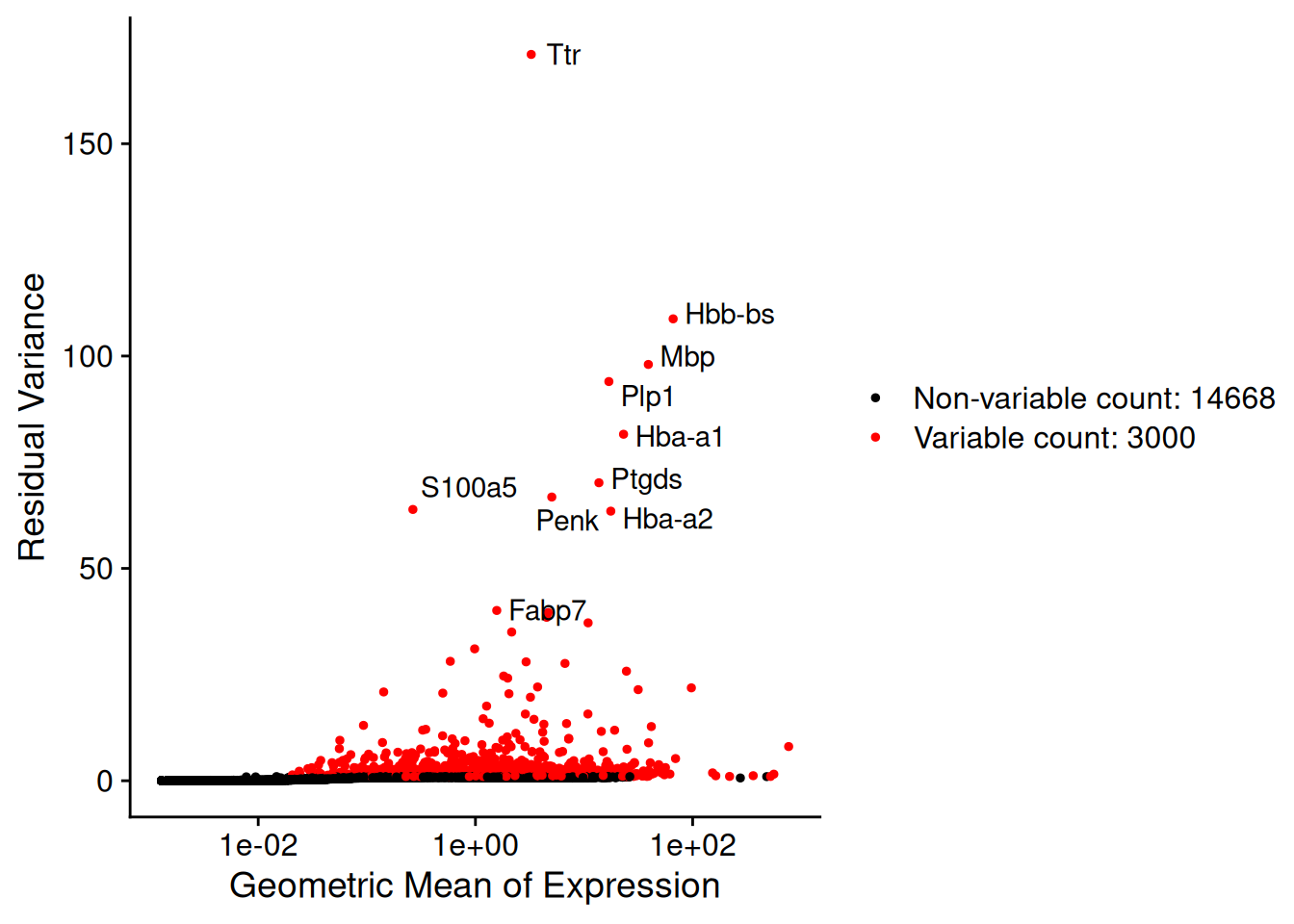

SpatialFeaturePlot(brain, features = c("Ttr","Hbb-bs"))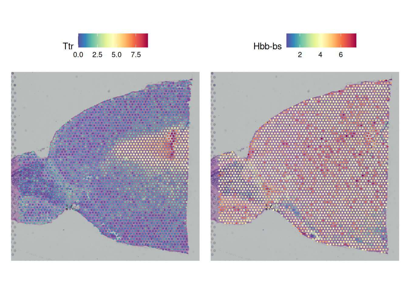

1.3 Réduction de dimension

brain <- RunPCA(brain, assay = "SCT", verbose = FALSE)
brain <- FindNeighbors(brain, reduction = "pca", dims = 1:30)

Computing nearest neighbor graph

Computing SNN

brain <- RunUMAP(brain, reduction = "pca", dims = 1:30)

Warning: The default method for RunUMAP has changed from calling Python UMAP via reticulate to the R-native UWOT using the cosine metric
To use Python UMAP via reticulate, set umap.method to 'umap-learn' and metric to 'correlation'
This message will be shown once per session

13:14:31 UMAP embedding parameters a = 0.9922 b = 1.112

13:14:31 Read 2696 rows and found 30 numeric columns

13:14:31 Using Annoy for neighbor search, n_neighbors = 30

13:14:31 Building Annoy index with metric = cosine, n_trees = 50

0%   10   20   30   40   50   60   70   80   90   100%

[----|----|----|----|----|----|----|----|----|----|

**************************************************|
13:14:31 Writing NN index file to temp file /tmp/RtmpZRDtDb/file5ed660a942a6
13:14:31 Searching Annoy index using 1 thread, search_k = 3000
13:14:32 Annoy recall = 100%
13:14:33 Commencing smooth kNN distance calibration using 1 thread with target n_neighbors = 30
13:14:36 Initializing from normalized Laplacian + noise (using RSpectra)
13:14:36 Commencing optimization for 500 epochs, with 105150 positive edges
13:14:36 Using rng type: pcg
13:14:41 Optimization finished

DimPlot(brain, reduction = "umap")+NoLegend()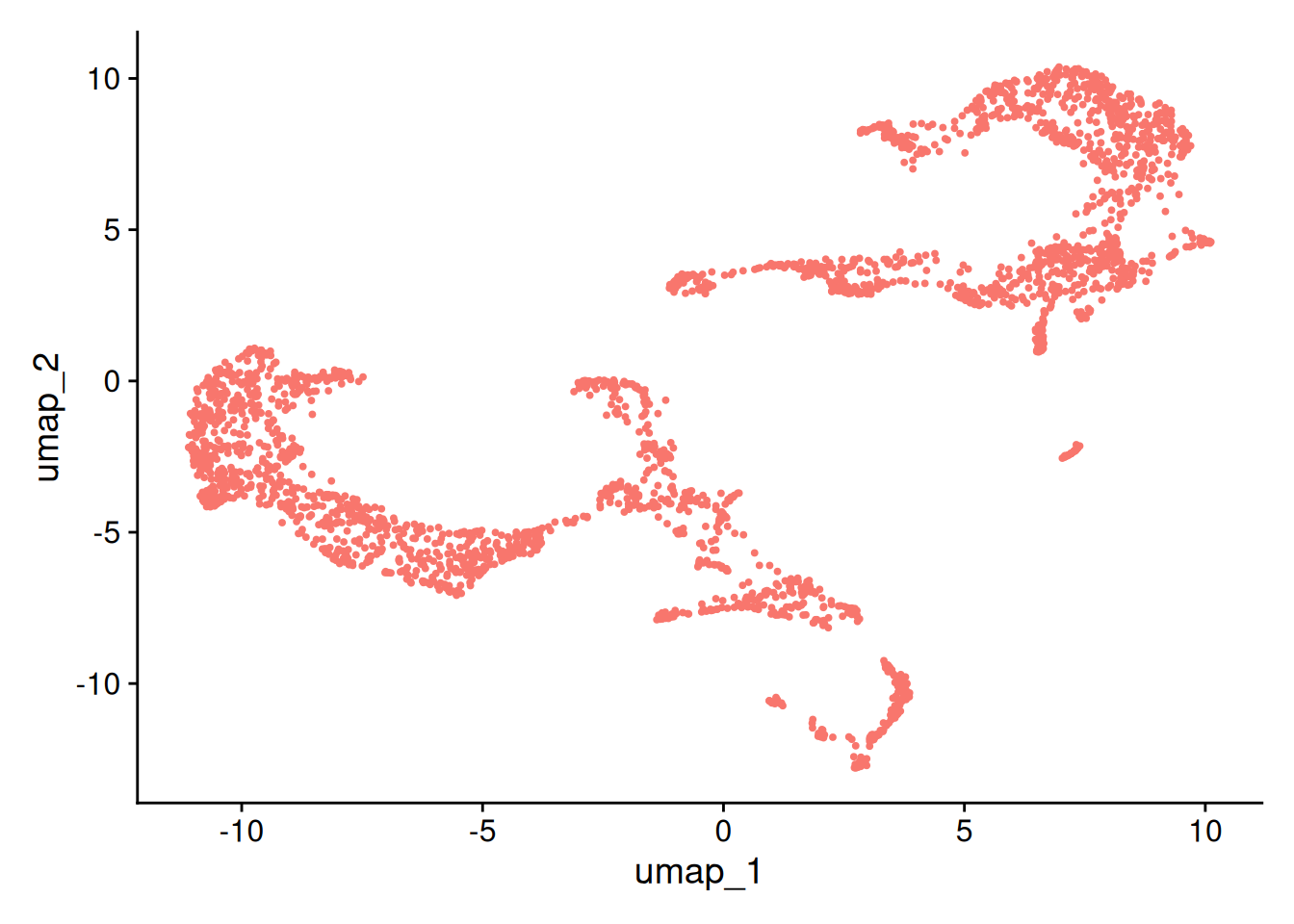

1.4 Clustering

Exemple avec BayesSpace

diet.seurat = Seurat::DietSeurat(brain,
                                   graphs = "SCT_nn",
                                   dimreducs = c("pca"))
sce_brain = as.SingleCellExperiment(diet.seurat, assay = "SCT") 
colData(sce_brain) = cbind(colData(sce_brain),
                           brain@images$anterior1$centroids@coords) 
sce_brain$array_col<-sce_brain$y 
sce_brain$array_row<-sce_brain$x 

sce_brain = spatialPreprocess(sce_brain, 
                          platform = "Visium",
                          skip.PCA = T, 
                          log.normalize = log.normalize) 
sce_brain <- spatialCluster(sce_brain,
                          nrep = 1000,
                          q= 8,
                          burn.in = 10,
                          model = "t",
                          gamma = 2)
brain@meta.data[["BayesSpace"]] <- as.factor(sce_brain$spatial.cluster)

EffPlot(brain,clustname="BayesSpace")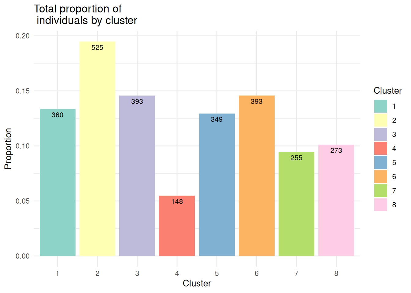

p1<-SpatialDimPlot(brain, "BayesSpace",label=TRUE,label.size=2)

Scale for fill is already present.
Adding another scale for fill, which will replace the existing scale.

p2<-DimPlot(brain, reduction = "umap",group.by="BayesSpace",label=TRUE)
p1+p2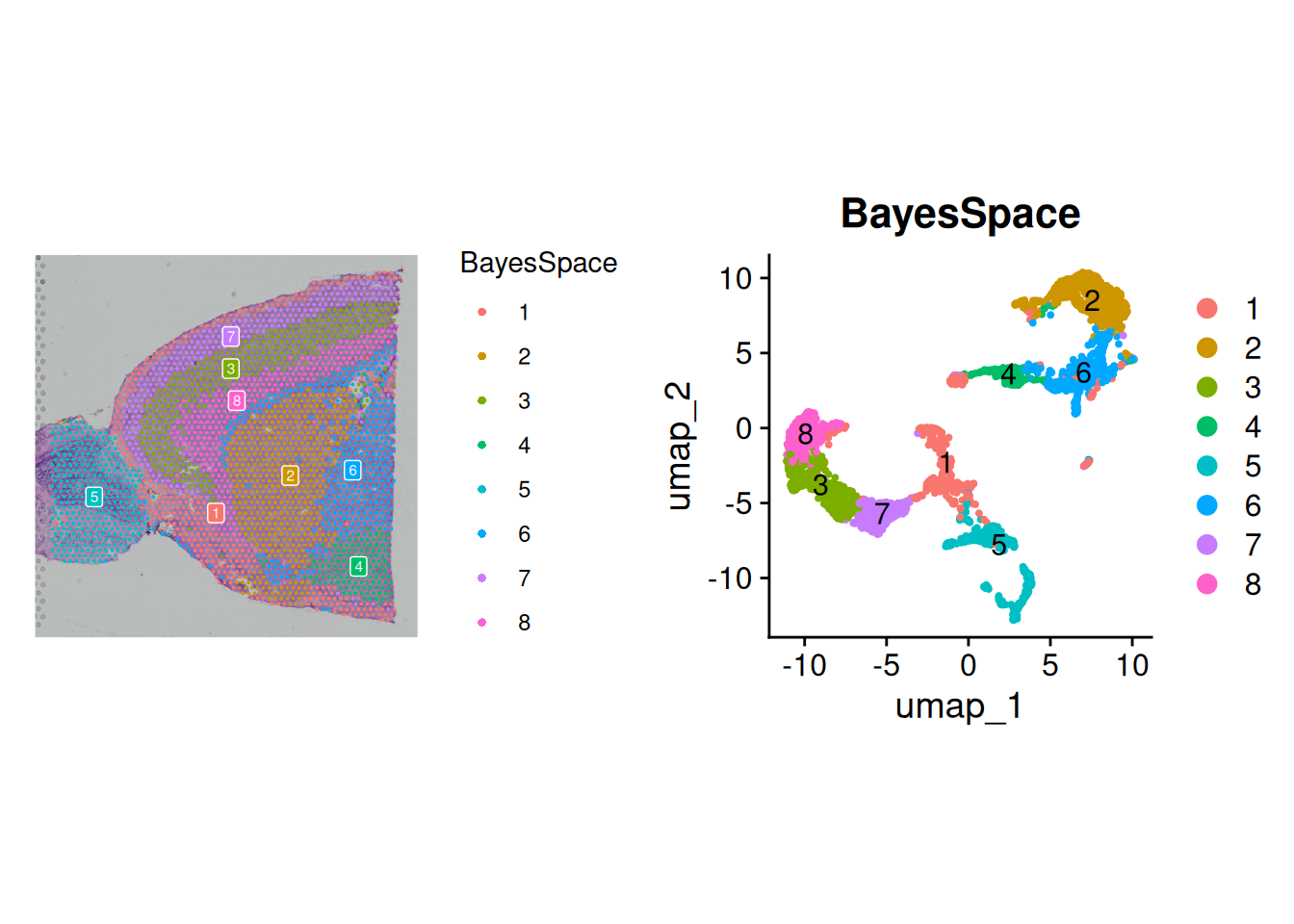

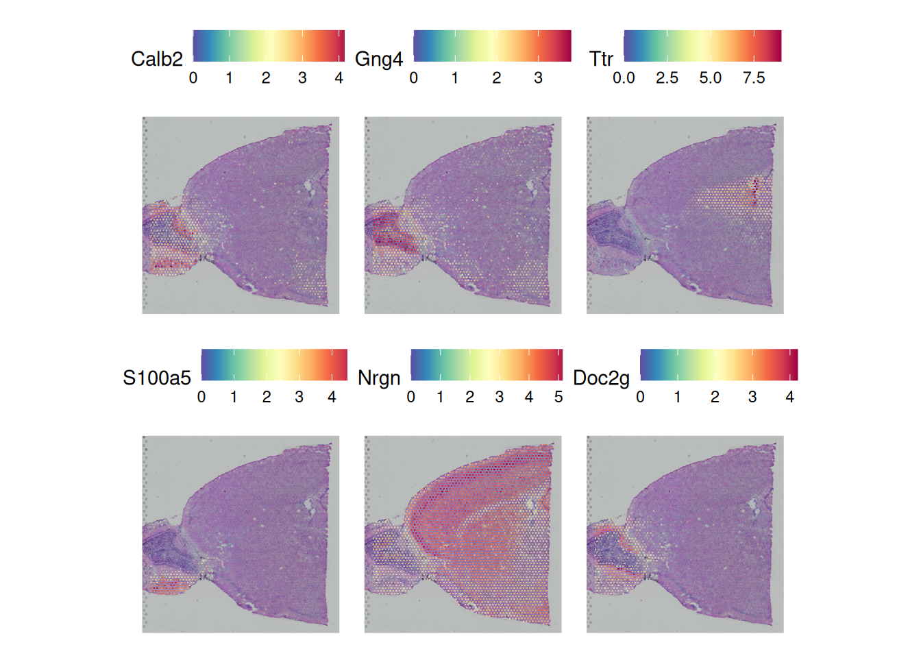
1.5 Spatial Variable Features

brain <- FindSpatiallyVariableFeatures(brain, 
                                       assay = "SCT", 
                                       features=VariableFeatures(brain)[1:1000],
                                       selection.method = "moransi")

top.features = rownames(
  dplyr::slice_min(
    brain[["SCT"]]@meta.features,
    moransi.spatially.variable.rank,
    n = 6
  )
)

SpatialFeaturePlot(brain, features = top.features, ncol = 3, alpha = c(0.1, 1))