library(Seurat)
library(ggplot2)
library(reshape2)
library(tidyverse)
library(DESeq2)
library(randomForest)
library(randomForestVIP)
library(ggvenn)
library(pheatmap)
library(clusterProfiler)
library(enrichplot)
library(org.Hs.eg.db)
source("Cours/FunctionsAux.R")TP - Partie 2
Analyse de deux conditions
1 Présentation et création de l’objet Seurat
1.1 Présentation des données
Les données
ifnbdisponibles dans seurat-dataDonnées de cellules sanguines humaines PBMC (Peripheral Blood Mononuclear Cells) dans deux conditions (stimulées par interférons/ contrôle). Les deux conditions sont indiquées dans la colonne
stimdes metadata de l’objet SO.
1.2 Objet Seurat depuis seurat data
SeuratData::InstallData("ifnb")
ifnb <- SeuratData::LoadData("ifnb")Assays(ifnb)An object of class "SimpleAssays"
Slot "data":
List of length 1Layers(ifnb) [1] "counts" "data" dim(ifnb) [1] 14053 13999table(ifnb$orig.ident)
IMMUNE_CTRL IMMUNE_STIM
6548 7451 table(ifnb$stim)
CTRL STIM
6548 7451
Remarque :
Dans Seurat V5 : un seul objet Seurat contenant les deux conditions, organisé en plusieurs “layers”
Dans les versions antérieures, un objet Seurat par condition
On splitte selon les deux conditions (counts.CTRL et counts.STIM)
ifnb[["RNA"]] <- split(ifnb[["RNA"]], f = ifnb$stim)
ifnb
An object of class Seurat
14053 features across 13999 samples within 1 assay
Active assay: RNA (14053 features, 0 variable features)
4 layers present: counts.CTRL, counts.STIM, data.CTRL, data.STIMdim(ifnb[["RNA"]]$counts.CTRL)[1] 14053 6548dim(ifnb[["RNA"]]$counts.STIM)[1] 14053 7451Une annotation des cellules est stockée dans meta.data$seurat_annotations :
head(ifnb@meta.data) orig.ident nCount_RNA nFeature_RNA stim seurat_annotations
AAACATACATTTCC.1 IMMUNE_CTRL 3017 877 CTRL CD14 Mono
AAACATACCAGAAA.1 IMMUNE_CTRL 2481 713 CTRL CD14 Mono
AAACATACCTCGCT.1 IMMUNE_CTRL 3420 850 CTRL CD14 Mono
AAACATACCTGGTA.1 IMMUNE_CTRL 3156 1109 CTRL pDC
AAACATACGATGAA.1 IMMUNE_CTRL 1868 634 CTRL CD4 Memory T
AAACATACGGCATT.1 IMMUNE_CTRL 1581 557 CTRL CD14 Mono1.3 Construction depuis les données de séquençage (?ifnb)
- Pour la récupération des données de séquençage, on a tout d’abord executé les commandes suivantes. Pour vous, elles sont déjà dans le dossier
data.
cd data/
wget https://www.dropbox.com/s/79q6dttg8yl20zg/immune_alignment_expression_matrices.zip
unzip immune_alignment_expression_matrices.zip
rm immune_alignment_expression_matrices.zip
# Lecture des deux fichiers de données
ctrl.data <- data.frame(data.table::fread('data/immune_control_expression_matrix.txt.gz',sep = "\t"),row.names=1)
stim.data <- data.frame(data.table::fread('data/immune_stimulated_expression_matrix.txt.gz',sep = "\t"),row.names=1)# Création de objet Seurat
ctrl <- Seurat::CreateSeuratObject(counts = ctrl.data, project = 'CTRL', min.cells = 5)
ctrl$stim <- 'CTRL'
ctrl <- subset(x = ctrl, subset = nFeature_RNA > 500)
stim <- Seurat::CreateSeuratObject(counts = stim.data, project = 'STIM', min.cells = 5)
stim$stim <- 'STIM'
stim <- subset(x = stim, subset = nFeature_RNA > 500)
ifnb2 <- merge(x = ctrl, y = stim)
Seurat::Project(object = ifnb2) <- 'ifnb'# Ajout de l'information d'annotation des cellules
annotations <- readRDS(file = system.file('extdata/annotations/annotations.Rds', package = 'ifnb.SeuratData'))
ifnb2 <- Seurat::AddMetaData(object = ifnb2, metadata = annotations)ifnbAn object of class Seurat
14053 features across 13999 samples within 1 assay
Active assay: RNA (14053 features, 0 variable features)
4 layers present: counts.CTRL, counts.STIM, data.CTRL, data.STIMifnb2An object of class Seurat
14053 features across 13999 samples within 1 assay
Active assay: RNA (14053 features, 0 variable features)
2 layers present: counts.CTRL, counts.STIMrm(ifnb2)2 Normalization, réduction de dimension et clustering
2.1 Normalisation
- Fait la normalisation comme vu précédemment pour chaque matrice de comptages (counts.CTRL –> data.CTRL et counts.STIM–> data.STIM)
ifnb <- NormalizeData(ifnb)Normalizing layer: counts.CTRLNormalizing layer: counts.STIMifnb@assays$RNA$data.CTRL[1:10,1:5]10 x 5 sparse Matrix of class "dgCMatrix"
AAACATACATTTCC.1 AAACATACCAGAAA.1 AAACATACCTCGCT.1
AL627309.1 . . .
RP11-206L10.2 . . .
LINC00115 . . .
NOC2L . . .
KLHL17 . . .
PLEKHN1 . . .
HES4 . . .
ISG15 . . 1.367106
AGRN . . .
C1orf159 . . .
AAACATACCTGGTA.1 AAACATACGATGAA.1
AL627309.1 . .
RP11-206L10.2 . .
LINC00115 . .
NOC2L . .
KLHL17 . .
PLEKHN1 . .
HES4 . .
ISG15 1.427573 .
AGRN . .
C1orf159 . .ifnb@assays$RNA$data.STIM[1:10,1:5]10 x 5 sparse Matrix of class "dgCMatrix"
AAACATACCAAGCT.1 AAACATACCCCTAC.1 AAACATACCCGTAA.1
AL627309.1 . . .
RP11-206L10.2 . . .
LINC00115 . . .
NOC2L . . .
KLHL17 . . .
PLEKHN1 . . .
HES4 . . .
ISG15 4.870775 4.982535 3.960974
AGRN . . .
C1orf159 . . .
AAACATACCCTCGT.1 AAACATACGAGGTG.1
AL627309.1 . .
RP11-206L10.2 . .
LINC00115 . .
NOC2L . .
KLHL17 . .
PLEKHN1 . .
HES4 . .
ISG15 3.902855 4.053323
AGRN . .
C1orf159 . . 2.2 HVG
- HVG : il le fait pour chaque condition puis rend une répondre globale et un graphe global
ifnb <- FindVariableFeatures(ifnb)Finding variable features for layer counts.CTRLFinding variable features for layer counts.STIMhead(VariableFeatures(ifnb,assay="RNA",layer="counts.CTRL"))[1] "HBB" "HBA2" "HBA1" "CCL3" "CCL4" "CXCL10"head(VariableFeatures(ifnb,assay="RNA",layer="counts.STIM"))[1] "HBB" "HBA2" "HBA1" "CCL4" "APOBEC3B" "CCL7" top10<-head(VariableFeatures(ifnb), 10)
plot1<-VariableFeaturePlot(ifnb)
plot2 <- LabelPoints(plot = plot1, points = top10, repel = TRUE)When using repel, set xnudge and ynudge to 0 for optimal resultsplot2Warning in scale_x_log10(): log-10 transformation introduced infinite values.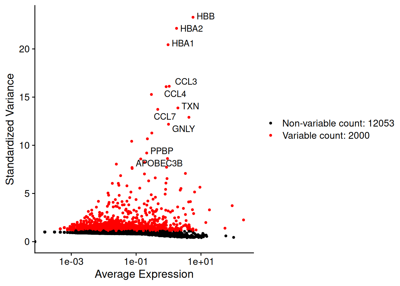
2.3 Réduction de dimension sans intégration
- Réduction de dimension sur la matrice des comptages normalisés (composée de deux blocs) centrés réduits
ifnb <- ScaleData(ifnb)Centering and scaling data matrixdim(ifnb@assays$RNA$scale.data)[1] 2000 13999ifnb <- RunPCA(ifnb)PC_ 1
Positive: NPM1, CCR7, GIMAP7, LTB, CD7, SELL, CD2, TMSB4X, TRAT1, IL7R
IL32, RHOH, ITM2A, RGCC, LEF1, CD3G, ALOX5AP, CREM, NHP2, PASK
MYC, SNHG8, TSC22D3, GPR171, BIRC3, NOP58, RARRES3, CD27, SRM, CD8B
Negative: TYROBP, C15orf48, FCER1G, CST3, SOD2, ANXA5, FTL, TYMP, TIMP1, CD63
LGALS1, CTSB, S100A4, LGALS3, KYNU, PSAP, FCN1, NPC2, ANXA2, S100A11
IGSF6, LYZ, SPI1, APOBEC3A, CD68, CTSL, SDCBP, NINJ1, HLA-DRA, CCL2
PC_ 2
Positive: ISG15, ISG20, IFIT3, IFIT1, LY6E, TNFSF10, IFIT2, MX1, IFI6, RSAD2
CXCL10, OAS1, CXCL11, IFITM3, MT2A, OASL, TNFSF13B, IDO1, IL1RN, APOBEC3A
GBP1, CCL8, HERC5, FAM26F, GBP4, HES4, WARS, VAMP5, DEFB1, XAF1
Negative: IL8, CLEC5A, CD14, VCAN, S100A8, IER3, MARCKSL1, IL1B, PID1, CD9
GPX1, PHLDA1, INSIG1, PLAUR, PPIF, THBS1, OSM, SLC7A11, GAPDH, CTB-61M7.2
LIMS1, S100A9, GAPT, CXCL3, ACTB, C19orf59, CEBPB, OLR1, MGST1, FTH1
PC_ 3
Positive: HLA-DQA1, CD83, HLA-DQB1, CD74, HLA-DPA1, HLA-DRA, HLA-DRB1, HLA-DPB1, SYNGR2, IRF8
CD79A, MIR155HG, HERPUD1, REL, HLA-DMA, MS4A1, HSP90AB1, FABP5, TVP23A, ID3
CCL22, EBI3, TSPAN13, PMAIP1, TCF4, PRMT1, NME1, HSPE1, HSPD1, CD70
Negative: ANXA1, GIMAP7, TMSB4X, CD7, CD2, RARRES3, MT2A, IL32, GNLY, PRF1
NKG7, CCL5, TRAT1, RGCC, S100A9, KLRD1, CCL2, GZMH, GZMA, CD3G
S100A8, CTSW, CCL7, ITM2A, HPSE, FGFBP2, CTSL, GPR171, CCL8, OASL
PC_ 4
Positive: CCR7, LTB, SELL, LEF1, IL7R, ADTRP, TRAT1, PASK, MYC, NPM1
SOCS3, TSC22D3, TSHZ2, HSP90AB1, SNHG8, GIMAP7, PIM2, HSPD1, CD3G, TXNIP
RHOH, GBP1, C12orf57, CA6, PNRC1, CMSS1, CD27, SESN3, NHP2, BIRC3
Negative: NKG7, GZMB, GNLY, CST7, CCL5, PRF1, CLIC3, KLRD1, GZMH, GZMA
APOBEC3G, CTSW, FGFBP2, KLRC1, FASLG, C1orf21, HOPX, CXCR3, SH2D1B, LINC00996
TNFRSF18, SPON2, RARRES3, GCHFR, SH2D2A, IGFBP7, ID2, C12orf75, XCL2, RAMP1
PC_ 5
Positive: VMO1, FCGR3A, MS4A4A, CXCL16, MS4A7, PPM1N, HN1, LST1, SMPDL3A, ATP1B3
CASP5, CDKN1C, CH25H, AIF1, PLAC8, SERPINA1, LRRC25, CD86, HCAR3, GBP5
TMSB4X, RP11-290F20.3, RGS19, VNN2, ADA, LILRA5, STXBP2, C3AR1, PILRA, FCGR3B
Negative: CCL2, CCL7, CCL8, PLA2G7, LMNA, S100A9, SDS, TXN, CSTB, ATP6V1F
CCR1, EMP1, CAPG, CCR5, TPM4, IDO1, MGST1, HPSE, CTSB, LILRB4
RSAD2, HSPA1A, VIM, CCNA1, CTSL, GCLM, PDE4DIP, SGTB, SLC7A11, FABP5 ifnb <- FindNeighbors(ifnb, dims = 1:30, reduction = "pca")Computing nearest neighbor graphComputing SNNifnb <- RunUMAP(ifnb, dims = 1:30, reduction = "pca", reduction.name = "umap.unintegrated")Warning: The default method for RunUMAP has changed from calling Python UMAP via reticulate to the R-native UWOT using the cosine metric
To use Python UMAP via reticulate, set umap.method to 'umap-learn' and metric to 'correlation'
This message will be shown once per session12:36:27 UMAP embedding parameters a = 0.9922 b = 1.11212:36:27 Read 13999 rows and found 30 numeric columns12:36:27 Using Annoy for neighbor search, n_neighbors = 3012:36:27 Building Annoy index with metric = cosine, n_trees = 500% 10 20 30 40 50 60 70 80 90 100%[----|----|----|----|----|----|----|----|----|----|**************************************************|
12:36:29 Writing NN index file to temp file /tmp/RtmpmRLL44/file38eb61c20997
12:36:29 Searching Annoy index using 1 thread, search_k = 3000
12:36:36 Annoy recall = 100%
12:36:37 Commencing smooth kNN distance calibration using 1 thread with target n_neighbors = 30
12:36:40 Initializing from normalized Laplacian + noise (using RSpectra)
12:36:41 Commencing optimization for 200 epochs, with 614378 positive edges
12:36:41 Using rng type: pcg
12:36:51 Optimization finishedDimPlot(ifnb, reduction = "umap.unintegrated", group.by = c("stim"))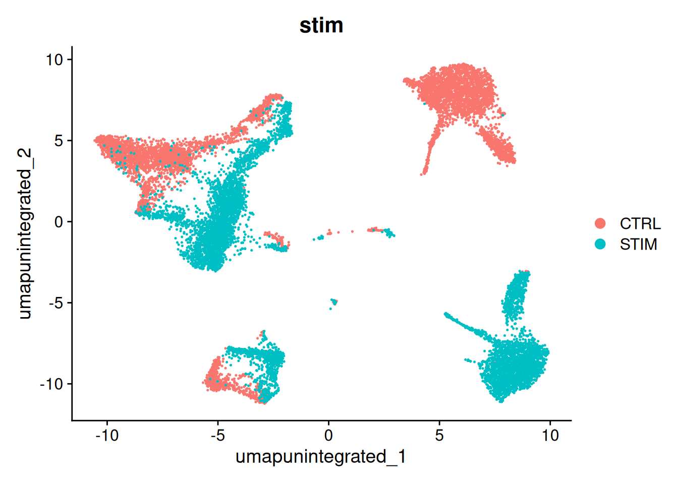
3 Intégration des données
3.1 Intégration avec CCA
- Utilisation de la fonction
IntegrateLayers()avec la méthode CCA = Canonical Correlation Analysis
ifnb_cca <- IntegrateLayers(object = ifnb,
                        method = CCAIntegration,
                        orig.reduction = "pca",
                        new.reduction = "integrated.cca",
                        verbose = FALSE)
# re-join layers after integration
ifnb_cca[["RNA"]] <- JoinLayers(ifnb_cca[["RNA"]])
# Dimension reduction
ifnb_cca <- FindNeighbors(ifnb_cca,
reduction = "integrated.cca",
dims = 1:30)Computing nearest neighbor graphComputing SNNifnb_cca <- RunUMAP(ifnb_cca,
dims = 1:30,
reduction = "integrated.cca")12:37:45 UMAP embedding parameters a = 0.9922 b = 1.11212:37:45 Read 13999 rows and found 30 numeric columns12:37:45 Using Annoy for neighbor search, n_neighbors = 3012:37:45 Building Annoy index with metric = cosine, n_trees = 500% 10 20 30 40 50 60 70 80 90 100%[----|----|----|----|----|----|----|----|----|----|**************************************************|
12:37:47 Writing NN index file to temp file /tmp/RtmpmRLL44/file38eb6ce693fe
12:37:47 Searching Annoy index using 1 thread, search_k = 3000
12:37:56 Annoy recall = 100%
12:37:57 Commencing smooth kNN distance calibration using 1 thread with target n_neighbors = 30
12:38:00 Initializing from normalized Laplacian + noise (using RSpectra)
12:38:00 Commencing optimization for 200 epochs, with 629246 positive edges
12:38:00 Using rng type: pcg
12:38:11 Optimization finishedp1<-DimPlot(ifnb, reduction = "umap.unintegrated", group.by = c("stim"))
p2<-DimPlot(ifnb_cca, reduction = "umap", group.by = c("stim"))
p1+p2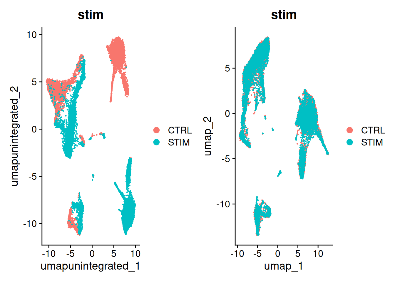
3.2 Intégration avec Harmony
ifnb_h <- IntegrateLayers(object = ifnb,
                        method = HarmonyIntegration,
                        orig.reduction = "pca",
                        new.reduction = "integrated.harmony",
                        verbose = FALSE)
# re-join layers after integration
ifnb_h[["RNA"]] <- JoinLayers(ifnb_h[["RNA"]])
# Dimension reduction
ifnb_h <- FindNeighbors(ifnb_h,
reduction = "integrated.harmony",
dims = 1:30)Computing nearest neighbor graphComputing SNNifnb_h <- RunUMAP(ifnb_h,
dims = 1:30,
reduction = "integrated.harmony")12:39:13 UMAP embedding parameters a = 0.9922 b = 1.11212:39:13 Read 13999 rows and found 30 numeric columns12:39:13 Using Annoy for neighbor search, n_neighbors = 3012:39:13 Building Annoy index with metric = cosine, n_trees = 500% 10 20 30 40 50 60 70 80 90 100%[----|----|----|----|----|----|----|----|----|----|**************************************************|
12:39:15 Writing NN index file to temp file /tmp/RtmpmRLL44/file38eb77da4176
12:39:15 Searching Annoy index using 1 thread, search_k = 3000
12:39:23 Annoy recall = 100%
12:39:25 Commencing smooth kNN distance calibration using 1 thread with target n_neighbors = 30
12:39:28 Initializing from normalized Laplacian + noise (using RSpectra)
12:39:28 Commencing optimization for 200 epochs, with 620048 positive edges
12:39:28 Using rng type: pcg
12:39:39 Optimization finishedp3<-DimPlot(ifnb_h, reduction = "umap", group.by = c("stim"))
p2+p3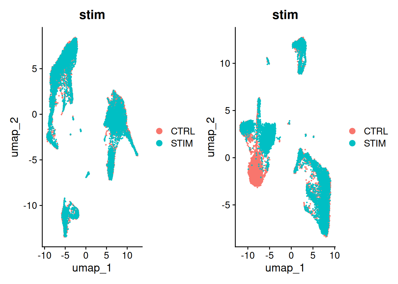
Pour la suite, on poursuit avec l’intégration par CCA
ifnb<-ifnb_cca
rm(ifnb_h,ifnb_cca)
4 Clustering
4.1 Méthode de Louvain
- Clustering sur les données intégrées avec la résolution \(r=0.5\)
#|message: false
#|warning: false

ifnb <- FindClusters(ifnb, resolution = 0.5)
Modularity Optimizer version 1.3.0 by Ludo Waltman and Nees Jan van Eck
Number of nodes: 13999
Number of edges: 590558
Running Louvain algorithm...
Maximum modularity in 10 random starts: 0.9021
Number of communities: 14
Elapsed time: 5 secondsEffPlot(ifnb,clustname = "seurat_clusters",resolution = 0.5)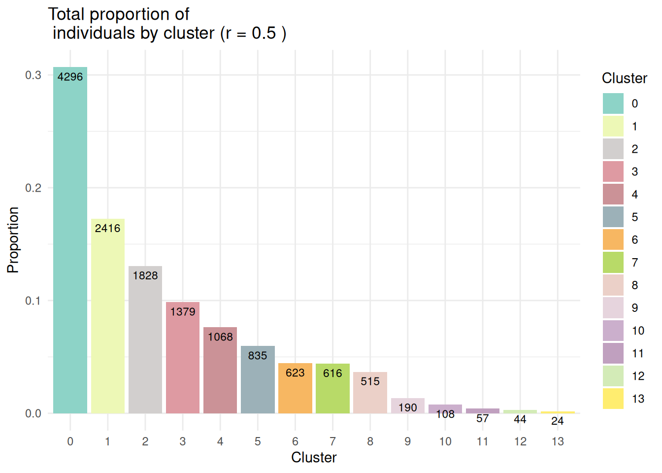
DimPlot(ifnb,
        reduction = "umap",
        group.by = c("stim", "seurat_clusters"))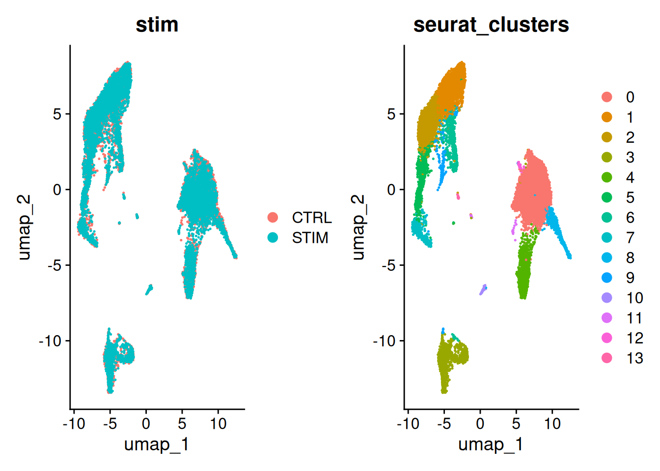
DimPlot(ifnb, reduction = "umap", split.by = "stim")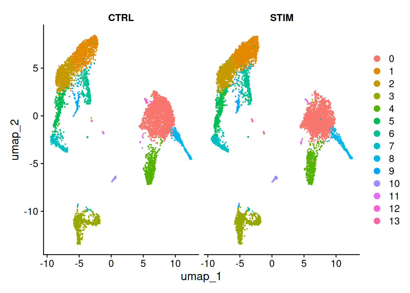
Aux<-melt(table(Idents(ifnb),ifnb$stim))
colnames(Aux)<-c("Cluster","Condition","len")
ggplot(data=Aux, aes(x=Cluster, y=len, fill=Condition)) +
  geom_bar(stat="identity", position=position_dodge())+
  geom_text(aes(label=len), vjust=1.6, color="white",
            position = position_dodge(0.9), size=3.5)+
  theme_minimal()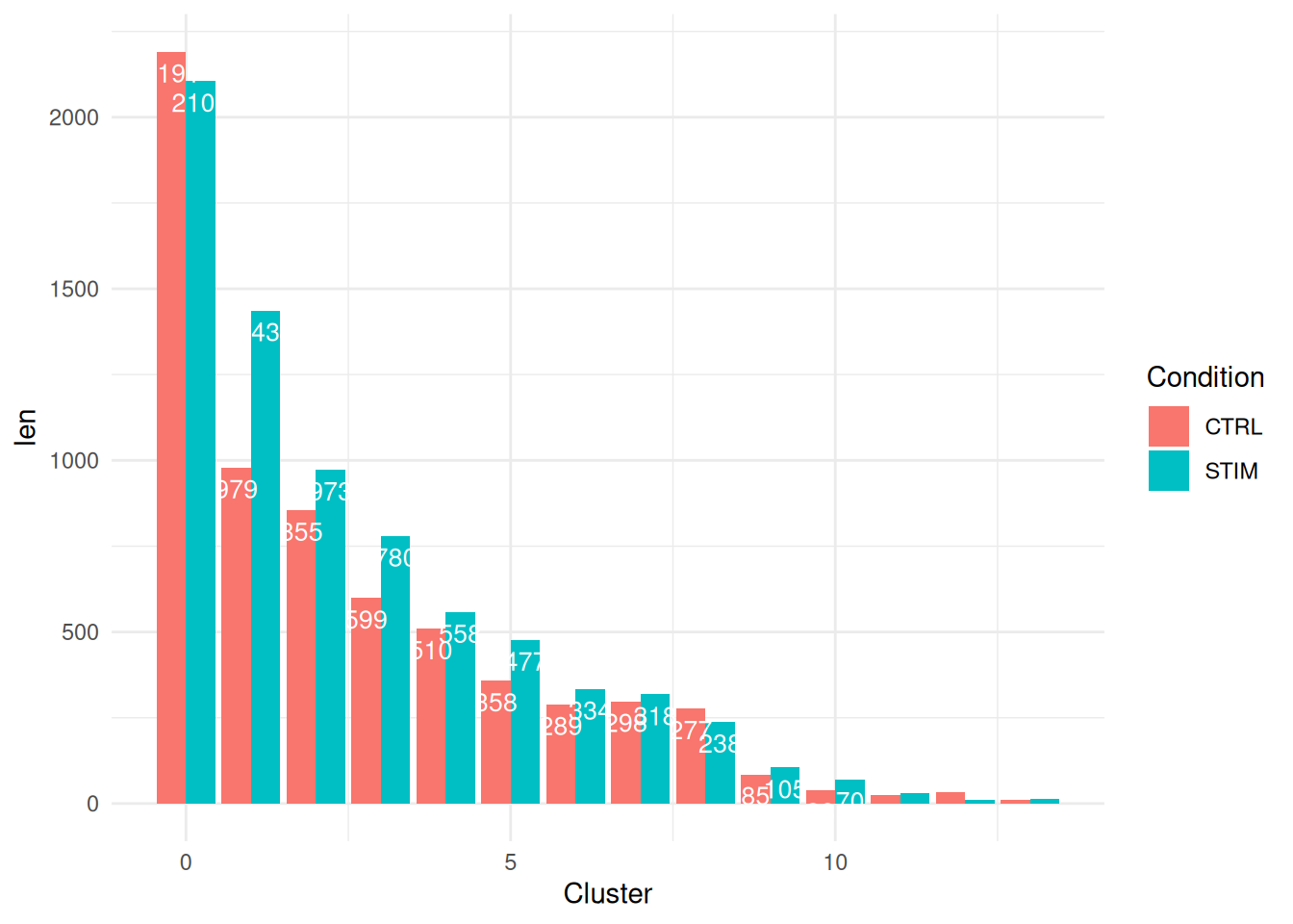
4.2 Annotation des cellules
- Une annotation des cellules est disponible
table(ifnb$seurat_annotations)
   CD14 Mono  CD4 Naive T CD4 Memory T    CD16 Mono            B        CD8 T
        4362         2504         1762         1044          978          814
 T activated           NK           DC  B Activated           Mk          pDC
         633          619          472          388          236          132
       Eryth
55 DimPlot(ifnb,
reduction = "umap",
group.by = c("seurat_annotations"))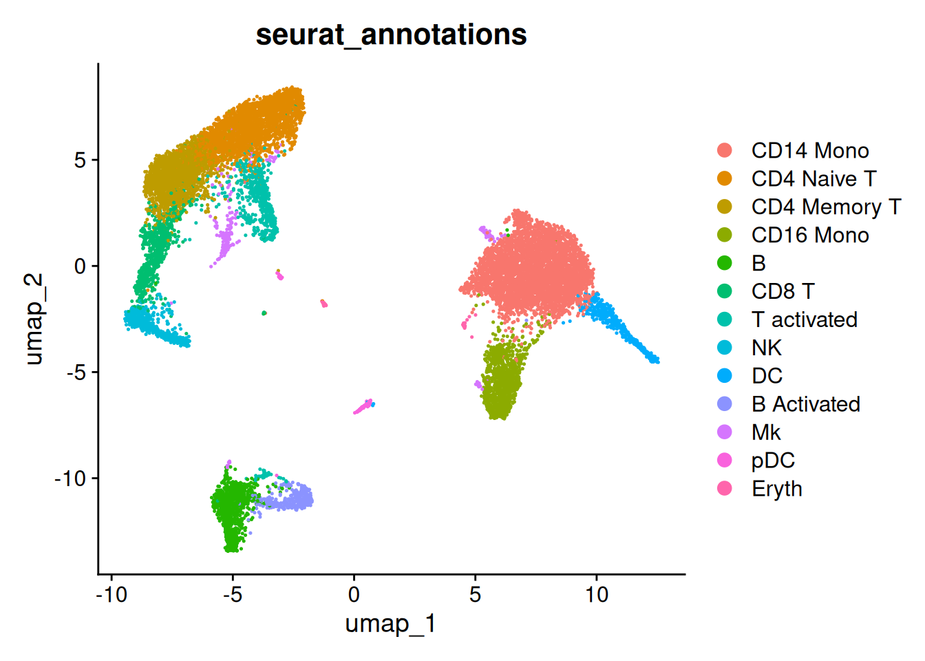
- Comparaison avec le clustering obtenu
table(Idents(ifnb),ifnb$seurat_annotations)[c(1:3,5,4,6:10,12,11,14,13),c(1:5,10,6:9,11:13)]
     CD14 Mono CD4 Naive T CD4 Memory T CD16 Mono    B B Activated CD8 T
  0       4272           0            0        16    1           1     0
  1          0        2332           47         1    1           0     9
  2          5         132         1643         0    0           0    30
  4         28           0            0      1027    0           0     0
  3          0           0            0         0  975         387     1
  5          1           2           51         0    0           0   765
  6          0          38            8         0    0           0     1
  7          0           0            0         0    0           0     8
  8         48           0            0         0    0           0     0
  9          0           0           13         0    1           0     0
  11         3           0            0         0    0           0     0
  10         0           0            0         0    0           0     0
  13         0           0            0         0    0           0     0
  12         5           0            0         0    0           0     0

     T activated   NK   DC   Mk  pDC Eryth
  0            0    0    4    2    0     0
  1           20    0    0    6    0     0
  2           16    1    0    1    0     0
  4            0    0    0   13    0     0
  3           15    0    0    0    0     1
  5            7    9    0    0    0     0
  6          575    0    0    0    1     0
  7            0  608    0    0    0     0
  8            0    0  466    0    1     0
  9            0    1    0  175    0     0
  11           0    0    0    0    0    54
  10           0    0    2    0  106     0
  13           0    0    0    0   24     0
  12           0    0    0   39    0     0
5 Gènes marqueurs des “types cellulaires” conservés
Déterminer les gènes marqueurs des “types cellulaires” qui sont conservés entre les conditions
Utilisation de la fonction
FindConservedMarkers()Exemple : on se focalise sur le type cellulaire NK
Idents(ifnb) <- "seurat_annotations"
NK.markers <- FindConservedMarkers(ifnb,
                                   ident.1 = "NK",
                                   grouping.var = "stim",
                                   verbose = FALSE)
head(NK.markers)
CTRL_p_val CTRL_avg_log2FC CTRL_pct.1 CTRL_pct.2 CTRL_p_val_adj
GNLY 0 6.854586 0.943 0.046 0
NKG7 0 5.358881 0.953 0.085 0
GZMB 0 5.078135 0.839 0.044 0
CLIC3 0 5.765314 0.601 0.024 0
CTSW 0 5.307246 0.537 0.030 0
KLRD1 0 5.261553 0.507 0.019 0
STIM_p_val STIM_avg_log2FC STIM_pct.1 STIM_pct.2 STIM_p_val_adj max_pval
GNLY 0 6.435910 0.956 0.059 0 0
NKG7 0 4.971397 0.950 0.081 0 0
GZMB 0 5.151924 0.897 0.060 0 0
CLIC3 0 5.505208 0.623 0.031 0 0
CTSW 0 5.240729 0.592 0.035 0 0
KLRD1 0 4.852457 0.555 0.027 0 0
minimump_p_val
GNLY 0
NKG7 0
GZMB 0
CLIC3 0
CTSW 0
KLRD1 0NK.markers<-NK.markers%>%
arrange(minimump_p_val)
DotPlot(ifnb, features = rownames(NK.markers)[1:10],
cols = c("blue", "red"), dot.scale = 8, split.by = "stim") +
RotatedAxis()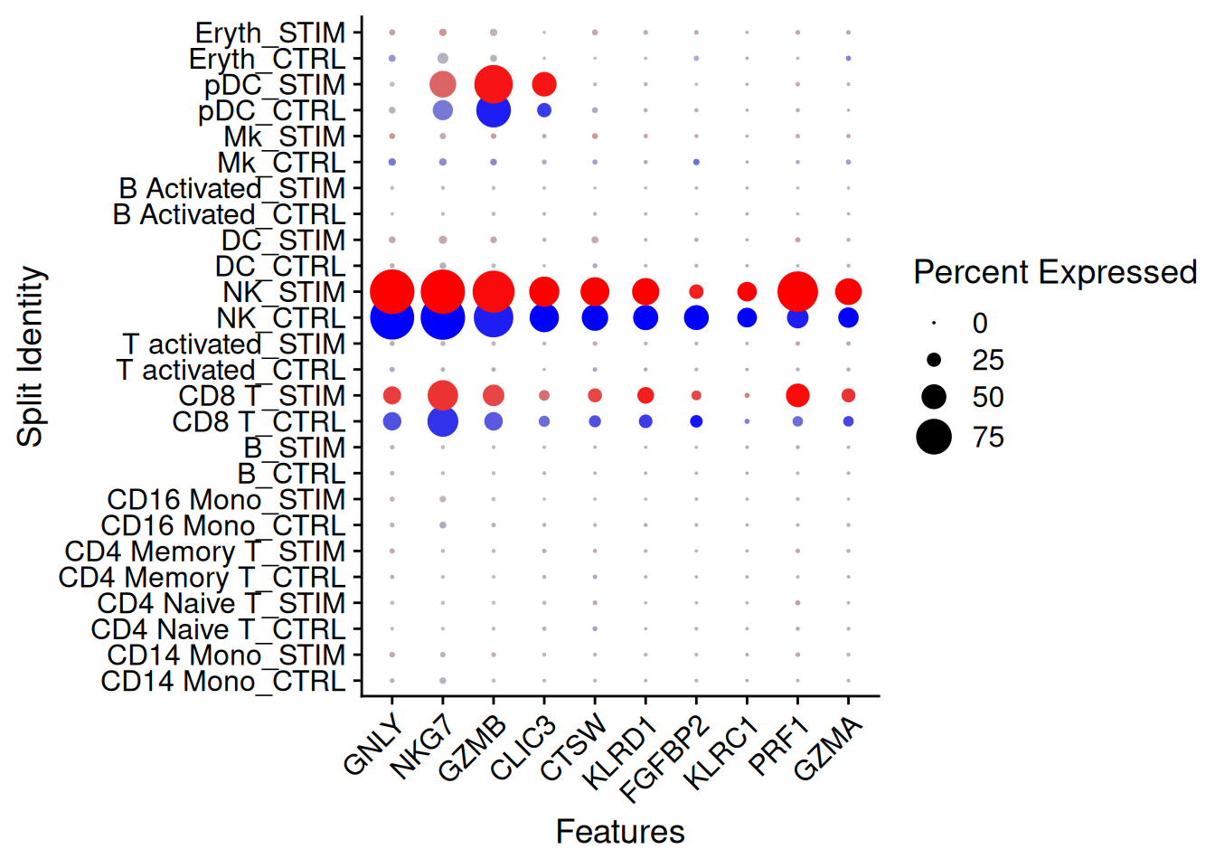
6 Analyse différentielle
6.1 Informations complémentaires
D’abord ajout d’informations complémentaires pour avoir des “réplicats”
# load the inferred sample IDs of each cell
ctrl <- read.table(url("https://raw.githubusercontent.com/yelabucsf/demuxlet_paper_code/master/fig3/ye1.ctrl.8.10.sm.best"), head = T, stringsAsFactors = F)
stim <- read.table(url("https://raw.githubusercontent.com/yelabucsf/demuxlet_paper_code/master/fig3/ye2.stim.8.10.sm.best"), head = T, stringsAsFactors = F)
info <- rbind(ctrl, stim)

# rename the cell IDs by substituting the '-' into '.'
info$BARCODE <- gsub(pattern = "\\-", replacement = "\\.", info$BARCODE)

# only keep the cells with high-confidence sample ID
info <- info[grep(pattern = "SNG", x = info$BEST), ]

# remove cells with duplicated IDs in both ctrl and stim groups
info <- info[!duplicated(info$BARCODE) & !duplicated(info$BARCODE, fromLast = T), ]

# now add the sample IDs to ifnb
rownames(info) <- info$BARCODE
info <- info[, c("BEST"), drop = F]
names(info) <- c("donor_id")
ifnb <- AddMetaData(ifnb, metadata = info)

# remove cells without donor IDs
ifnb$donor_id[is.na(ifnb$donor_id)] <- "unknown"
ifnb <- subset(ifnb, subset = donor_id != "unknown")table(ifnb$donor_id)
 SNG-101 SNG-1015 SNG-1016 SNG-1039  SNG-107 SNG-1244 SNG-1256 SNG-1488
    1197     3116     1438      663      652     1998     2363     2241
Pour la suite, création d’une colonne celltype.stim combinant le type cellulaire et la condition.
ifnb$celltype.stim <- paste(ifnb$seurat_annotations, ifnb$stim, sep = "_")
table(ifnb$celltype.stim)
 B Activated_CTRL  B Activated_STIM            B_CTRL            B_STIM
              176               198               403               554
   CD14 Mono_CTRL    CD14 Mono_STIM    CD16 Mono_CTRL    CD16 Mono_STIM
             2167              2086               494               521
CD4 Memory T_CTRL CD4 Memory T_STIM  CD4 Naive T_CTRL  CD4 Naive T_STIM
              849               876               960              1497
       CD8 T_CTRL        CD8 T_STIM           DC_CTRL           DC_STIM
              349               451               255               208
       Eryth_CTRL        Eryth_STIM           Mk_CTRL           Mk_STIM
               22                32               110               114
          NK_CTRL           NK_STIM          pDC_CTRL          pDC_STIM
              295               310                49                79
 T activated_CTRL  T activated_STIM
              291               322
Création d’une colonne donor.stim combinant le donneur et la condition
ifnb$donor.stim<-paste0(ifnb$donor_id,"_",ifnb$stim)6.2 Exemple 1
Question 1: déterminer les gènes dont l’expression varie entre les deux conditions (types cellulaires confondus)
6.2.1 Par méthode naive (Wilcoxon)
Idents(ifnb)<-ifnb$stim
res1_Wilcox <- FindMarkers(object = ifnb,
                           ident.1 = "STIM",
                           ident.2 = "CTRL",
                           test.use = "wilcox")

sum(res1_Wilcox$p_val_adj<0.01)
[1] 2384round(100*mean(res1_Wilcox$p_val_adj<0.01),2)[1] 34.67genetop_wilcox1<-res1_Wilcox %>%
filter(p_val_adj<0.01)%>%
arrange(desc(abs(avg_log2FC)))%>%
top_n(200)DotPlot(ifnb,features=rownames(genetop_wilcox1)[1:10],group.by="stim")+
theme(axis.text.x = element_text(angle = 90, vjust = 0.5, hjust=1))Warning: Scaling data with a low number of groups may produce misleading
results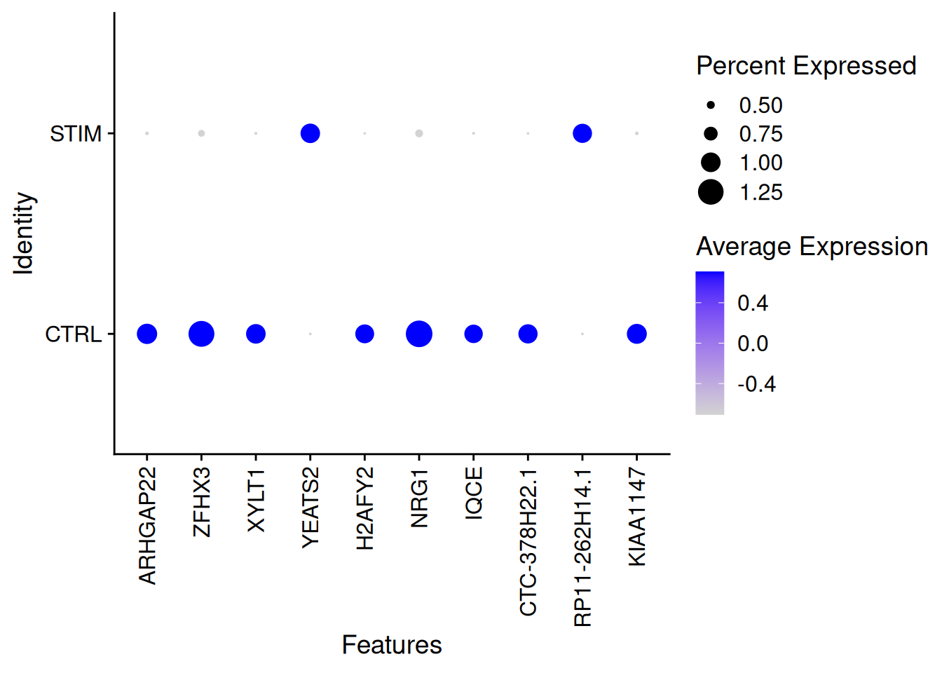
DotPlot(ifnb,features=rownames(genetop_wilcox1)[1:10],group.by="celltype.stim")+
  theme(axis.text.x = element_text(angle = 90, vjust = 0.5, hjust=1))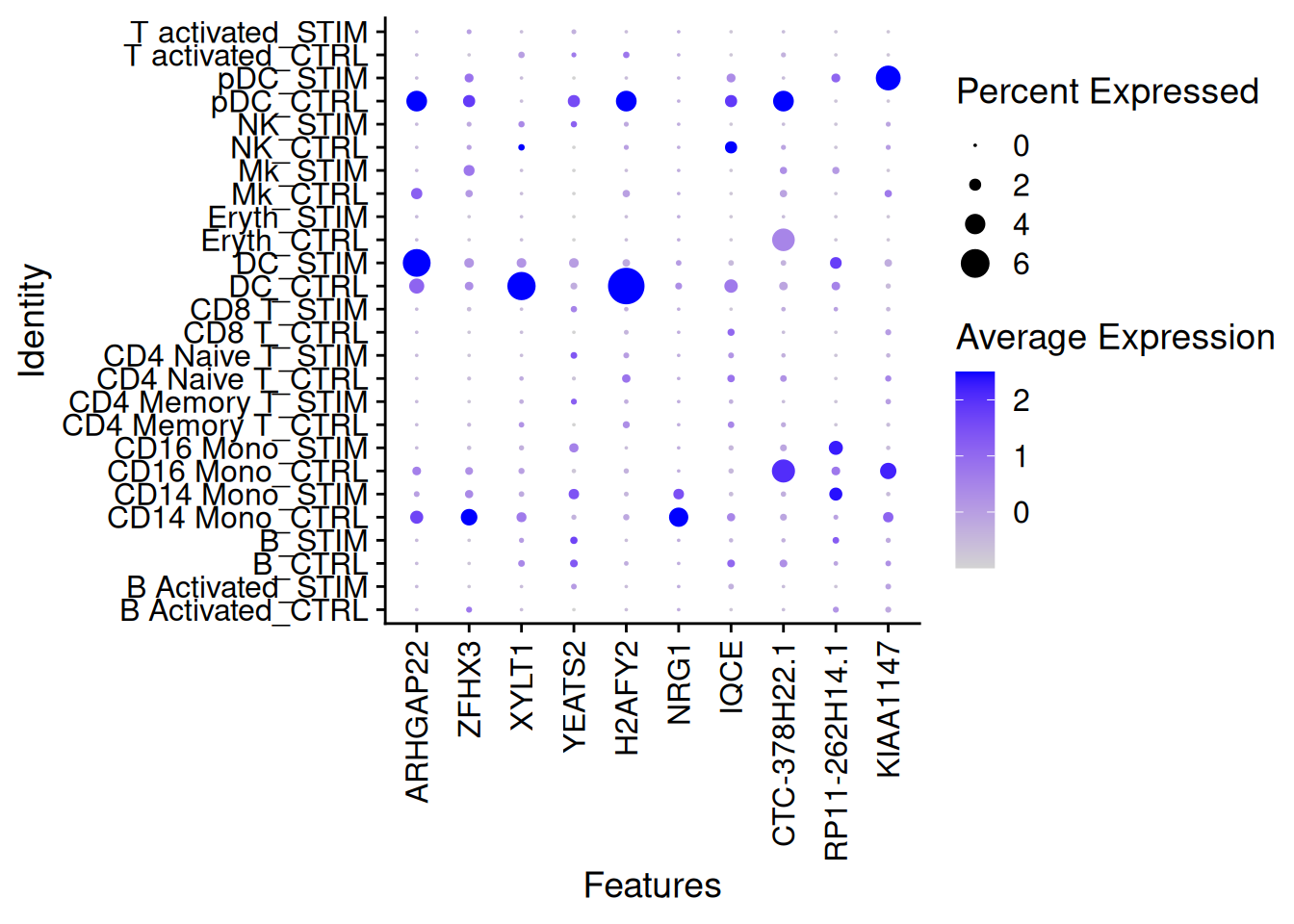
6.2.2 Par pseudo-bulk (DESeq2)
- On regroupe par condition et donor_id pour la création des données de pseudoBulk
pseudo_ifnb1 <- AggregateExpression(ifnb,
                                   assays = "RNA",
                                   return.seurat = T,
                                   group.by = c("stim", "donor_id"))
Centering and scaling data matrixhead(pseudo_ifnb1) orig.ident stim donor_id
CTRL_SNG-101 CTRL_SNG-101 CTRL SNG-101
CTRL_SNG-1015 CTRL_SNG-1015 CTRL SNG-1015
CTRL_SNG-1016 CTRL_SNG-1016 CTRL SNG-1016
CTRL_SNG-1039 CTRL_SNG-1039 CTRL SNG-1039
CTRL_SNG-107 CTRL_SNG-107 CTRL SNG-107
CTRL_SNG-1244 CTRL_SNG-1244 CTRL SNG-1244
CTRL_SNG-1256 CTRL_SNG-1256 CTRL SNG-1256
CTRL_SNG-1488 CTRL_SNG-1488 CTRL SNG-1488
STIM_SNG-101 STIM_SNG-101 STIM SNG-101
STIM_SNG-1015 STIM_SNG-1015 STIM SNG-1015- DESeq2 depuis Seurat
Idents(pseudo_ifnb1)<-"stim"
bulk.cond1 <- FindMarkers(object = pseudo_ifnb1,
                         ident.1 = "STIM",
                         ident.2 = "CTRL",
                         test.use = "DESeq2")
converting counts to integer modegene-wise dispersion estimatesmean-dispersion relationshipfinal dispersion estimateshead(bulk.cond1) p_val avg_log2FC pct.1 pct.2 p_val_adj
NT5C3A 7.029232e-232 3.554826 1 1 9.878179e-228
IFI16 5.065325e-212 2.243370 1 1 7.118302e-208
ISG20 2.122045e-205 4.018798 1 1 2.982110e-201
DDX58 1.126106e-175 3.548703 1 1 1.582516e-171
RTP4 6.577415e-171 2.989407 1 1 9.243241e-167
TRIM22 1.565830e-162 2.864154 1 1 2.200461e-158- En passant par le package DESeq2
cts1<-as.matrix(pseudo_ifnb1@assays$RNA$counts)
coldata1<-pseudo_ifnb1@meta.data
dds1 <- DESeqDataSetFromMatrix(countData = cts1,
                              colData = coldata1,
                              design= ~ donor_id + stim)
dds1 <- DESeq(dds1,fitType = c("local"))
resultsNames(dds1) # lists the coefficients
[1] "Intercept" "donor_id_SNG.1015_vs_SNG.101"
[3] "donor_id_SNG.1016_vs_SNG.101" "donor_id_SNG.1039_vs_SNG.101"
[5] "donor_id_SNG.107_vs_SNG.101" "donor_id_SNG.1244_vs_SNG.101"
[7] "donor_id_SNG.1256_vs_SNG.101" "donor_id_SNG.1488_vs_SNG.101"
[9] "stim_STIM_vs_CTRL" resDEseq1<-results(dds1,name="stim_STIM_vs_CTRL")
round(100*length(which(resDEseq1$padj<0.01))/nrow(resDEseq1),2) [1] 17.47genetopDEseq1<-as.data.frame(resDEseq1) %>%
filter(padj<0.01)%>%
arrange(desc(abs(log2FoldChange)))%>%
top_n(200)Selecting by padjDotPlot(pseudo_ifnb1,features=rownames(genetopDEseq1)[1:10],group.by="stim")+
theme(axis.text.x = element_text(angle = 90, vjust = 0.5, hjust=1))Warning: Scaling data with a low number of groups may produce misleading
results
DotPlot(ifnb,features=rownames(genetopDEseq1)[1:10],group.by="stim")+
  theme(axis.text.x = element_text(angle = 90, vjust = 0.5, hjust=1))
Warning: Scaling data with a low number of groups may produce misleading
results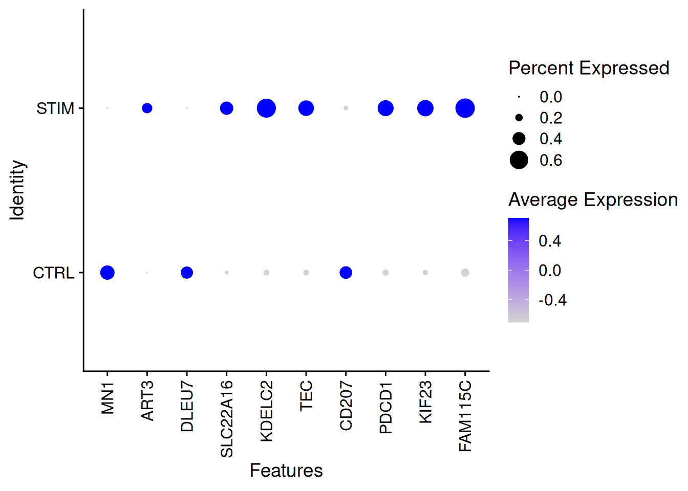
pheatmap(pseudo_ifnb1@assays$RNA$scale.data[rownames(genetopDEseq1),],
         cluster_cols = FALSE,
         scale = "column",
         show_rownames = FALSE,
         show_colnames = TRUE)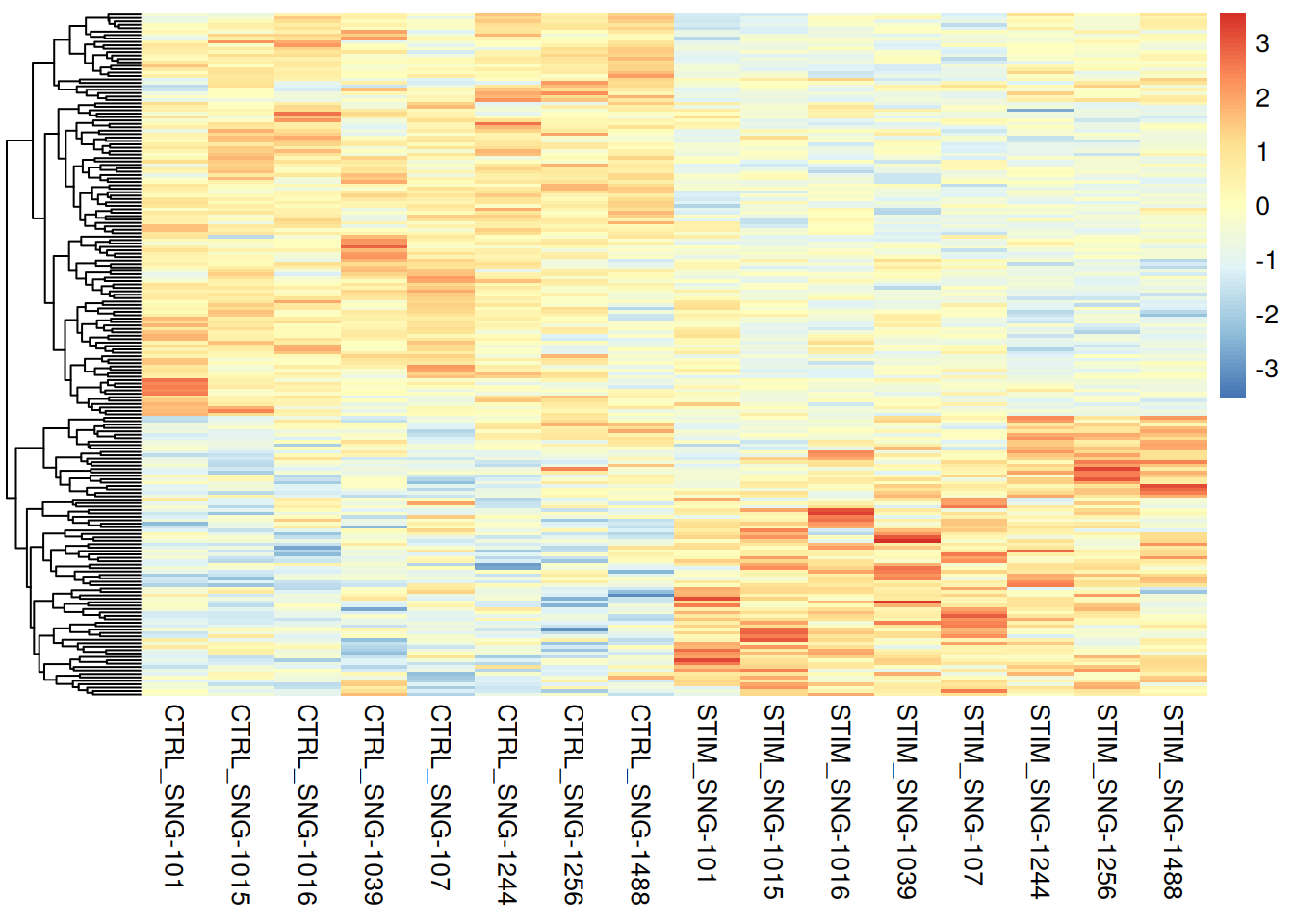
6.2.3 Par une méthode spécifique single-cell (ex: NEBULA)
library(nebula)
ifnb_neb1<-scToNeb(obj=ifnb,assay="RNA",id="donor_id",pred=c("stim","seurat_annotations"))
df1 = model.matrix(~stim+seurat_annotations, data=ifnb_neb1$pred)
data_g = group_cell(count=ifnb_neb1$count,id=ifnb_neb1$id,pred=df1) # il faut grouper les cellules par indiv avant de faire nebula
#re1 = nebula(data_g$count,data_g$id,pred=data_g$pred)
re1<-readRDS("Exercices/ResNebulaQ1.rds")
round(100*mean(p.adjust(re1$summary$p_stimSTIM,method="BH")<0.01),2)[1] 49.1ifnbNebSumm1<-re1$summary
ifnbNebSumm1$padjStim<-p.adjust(re1$summary$p_stimSTIM,method="BH")
ifnbNebSumm1<-ifnbNebSumm1%>%
filter(padjStim <0.01)%>%
arrange(desc(abs(logFC_stimSTIM)))
head(ifnbNebSumm1) logFC_(Intercept) logFC_stimSTIM logFC_seurat_annotationsCD4 Naive T
1 -3.0231869 6.387177 -5.955392
2 -3.4110331 5.913719 -5.838174
3 -0.6599773 5.293059 -4.835198
4 -5.8264308 5.277627 -2.160834
5 -6.5605195 5.195983 -5.509365
6 -8.9263424 4.943081 -5.356895
logFC_seurat_annotationsCD4 Memory T logFC_seurat_annotationsCD16 Mono
1 -5.5038664 -2.43210273
2 -5.4847981 -0.18167624
3 -4.6971026 1.39648553
4 -0.4273964 0.34525472
5 -4.7460927 -0.02139147
6 -5.5182972 -2.57423478
logFC_seurat_annotationsB logFC_seurat_annotationsCD8 T
1 -5.829592 -5.937029
2 -3.103156 -5.441283
3 -2.371866 -5.481890
4 -3.952811 -2.094269
5 -4.301807 -4.791603
6 -5.050143 -20.136702
logFC_seurat_annotationsT activated logFC_seurat_annotationsNK
1 -5.819184 -5.371862
2 -5.476636 -5.791665
3 -3.136328 -5.336081
4 -2.961456 -3.402649
5 -19.491487 -5.131678
6 -20.047400 -20.101178
logFC_seurat_annotationsDC logFC_seurat_annotationsB Activated
1 -2.59802435 -4.942419
2 0.47567977 -2.465261
3 0.08834702 -1.994659
4 0.58122480 -18.227450
5 0.25232950 -4.651815
6 -0.31818241 -1.900209
logFC_seurat_annotationsMk logFC_seurat_annotationspDC
1 -2.287668 -5.61437729
2 -2.220169 -2.69192426
3 -1.687551 -1.92545848
4 -1.226571 0.00605799
5 -1.670717 -0.46379865
6 -2.357705 -3.04958468
logFC_seurat_annotationsEryth se_(Intercept) se_stimSTIM
1 -1.674200 0.40184447 0.08563252
2 -1.514332 0.09623187 0.11141246
3 -1.432106 0.05063235 0.05214685
4 -1.150273 24.90068402 0.50189670
5 -1.097119 36.39034351 0.33471753
6 -1.118504 120.18996859 0.45268993
se_seurat_annotationsCD4 Naive T se_seurat_annotationsCD4 Memory T
1 0.09080246 0.09750737
2 0.15805632 0.16873458
3 0.06314074 0.07421262
4 0.19506552 0.11763804
5 0.57898811 0.50156695
6 0.71298736 1.00429979
se_seurat_annotationsCD16 Mono se_seurat_annotationsB
1 0.07969934 0.13337741
2 0.04792581 0.07658355
3 0.06692279 0.07115839
4 0.11110584 0.71063771
5 0.07474477 0.50181858
6 0.32102251 1.00568863
se_seurat_annotationsCD8 T se_seurat_annotationsT activated
1 0.1578810 1.747862e-01
2 0.2289437 2.829292e-01
3 0.1187099 9.415266e-02
4 0.3106483 5.829233e-01
5 0.7085561 8.113770e+02
6 1299.0548676 1.475353e+03
se_seurat_annotationsNK se_seurat_annotationsDC
1 0.1513727 0.11611478
2 0.3213261 0.06749747
3 0.1371742 0.08497132
4 0.7116677 0.15267928
5 1.0011740 0.10159948
6 1479.0206709 0.21714832
se_seurat_annotationsB Activated se_seurat_annotationsMk
1 0.1657077 0.1523154
2 0.1021583 0.1248050
3 0.1072164 0.1481700
4 909.9582229 0.4231231
5 1.0015331 0.3089855
6 0.3889408 0.6117675
se_seurat_annotationspDC se_seurat_annotationsEryth p_(Intercept)
1 0.3217026 0.2760968 5.342043e-14
2 0.1719185 0.1970072 3.345229e-275
3 0.1715396 0.2515428 7.767610e-39
4 0.2970370 0.7316917 8.149952e-01
5 0.2150128 0.4238227 8.569313e-01
6 1.0290549 0.6833769 9.407967e-01
p_stimSTIM p_seurat_annotationsCD4 Naive T p_seurat_annotationsCD4 Memory T
1 0.000000e+00 0.000000e+00 0.000000e+00
2 0.000000e+00 1.164713e-298 8.922565e-232
3 0.000000e+00 0.000000e+00 0.000000e+00
4 7.339587e-26 1.613556e-28 2.799844e-04
5 2.406183e-54 1.808304e-21 3.005789e-21
6 9.315778e-28 5.765069e-14 3.914389e-08
p_seurat_annotationsCD16 Mono p_seurat_annotationsB p_seurat_annotationsCD8 T
1 1.600099e-204 0.000000e+00 1.817356e-309
2 1.501744e-04 0.000000e+00 7.347369e-125
3 1.065760e-96 1.318880e-243 0.000000e+00
4 1.887155e-03 2.661755e-08 1.566451e-11
5 7.747299e-01 1.013205e-17 1.356407e-11
6 1.067305e-15 5.124893e-07 9.876325e-01
p_seurat_annotationsT activated p_seurat_annotationsNK p_seurat_annotationsDC
1 4.850575e-243 7.622319e-276 6.954368e-111
2 1.782461e-83 1.256825e-72 1.823288e-12
3 2.667416e-243 0.000000e+00 2.984665e-01
4 3.767330e-07 1.742226e-06 1.407567e-04
5 9.808345e-01 2.964967e-07 1.300725e-02
6 9.891585e-01 9.891564e-01 1.428454e-01
p_seurat_annotationsB Activated p_seurat_annotationsMk
1 1.790624e-195 5.489659e-51
2 1.159895e-128 8.584632e-71
3 2.979775e-77 4.728367e-30
4 9.840186e-01 3.745330e-03
5 3.405813e-06 6.405090e-08
6 1.031141e-06 1.162403e-04
p_seurat_annotationspDC p_seurat_annotationsEryth gene_id gene padjStim
1 3.319516e-68 1.329305e-09 10969 CCL8 0.000000e+00
2 2.923012e-55 1.509971e-14 3282 CXCL11 0.000000e+00
3 3.088817e-29 1.246159e-08 3281 CXCL10 0.000000e+00
4 9.837285e-01 1.159334e-01 9199 TGM1 8.239827e-25
5 3.099986e-02 9.635954e-03 2620 HESX1 4.620373e-53
6 3.041807e-03 1.016869e-01 8963 CCNA1 1.100814e-26genetopNeb1<-ifnbNebSumm1%>%
top_n(200)Selecting by padjStimDotPlot(ifnb,features=genetopNeb1$gene[1:30],group.by="stim")+
theme(axis.text.x = element_text(angle = 90, vjust = 0.5, hjust=1))Warning: Scaling data with a low number of groups may produce misleading
results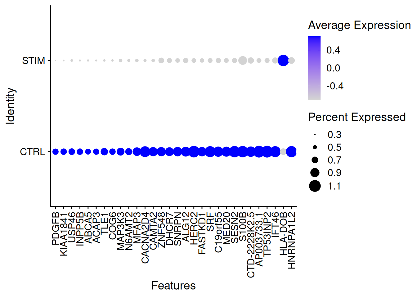
pheatmap(pseudo_ifnb1@assays$RNA$scale.data[genetopNeb1$gene,],
         cluster_cols = FALSE,
         scale = "column",
         show_rownames = FALSE,
         show_colnames = TRUE)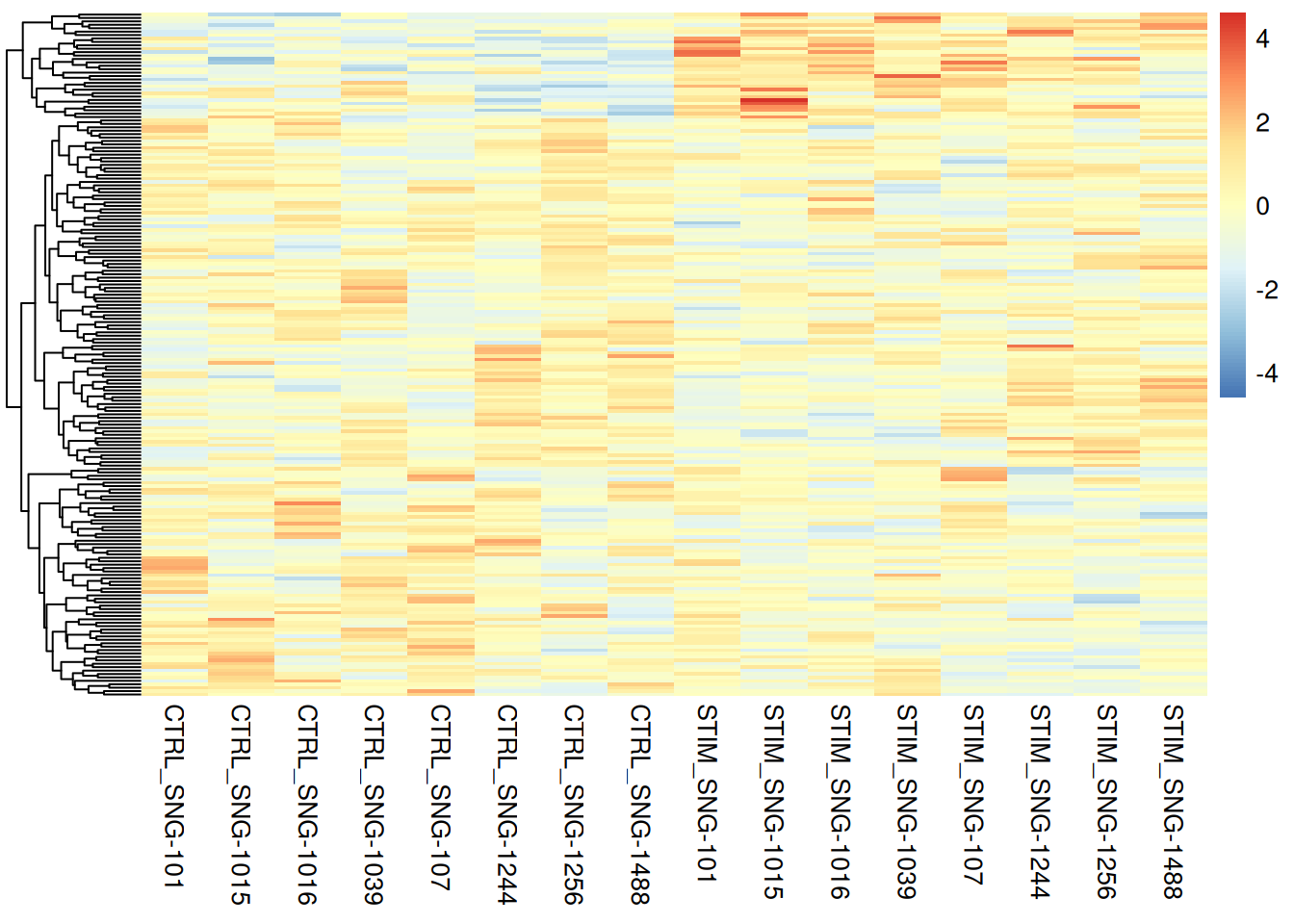
6.2.4 Comparaison
ggvenn(list(DEseq2=rownames(genetopDEseq1),
            Nebula=genetopNeb1$gene,
            Wilcox=rownames(genetop_wilcox1)))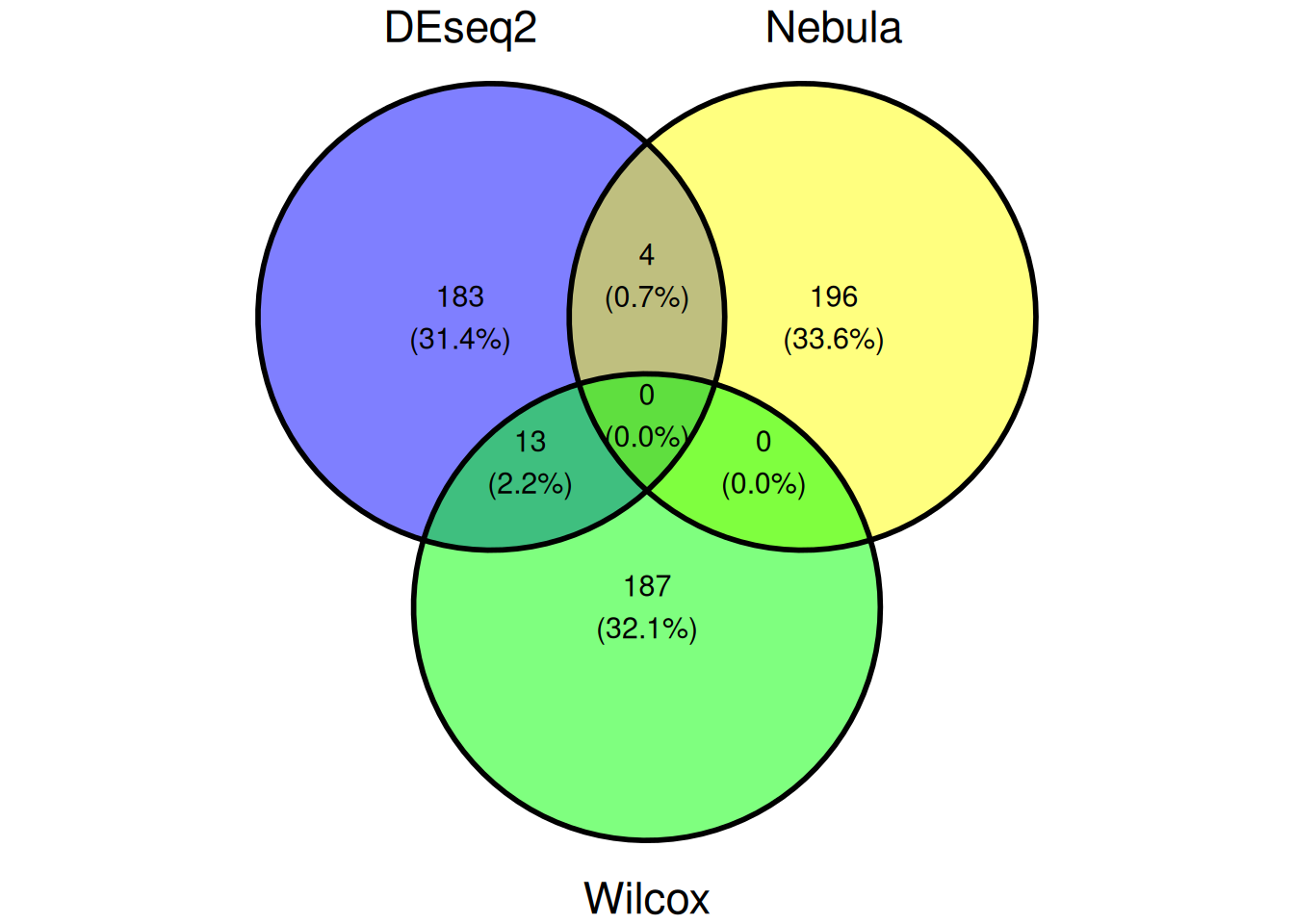
6.3 Exemple 2
Question 2 : déterminer les gènes dont l’expression varie entre les deux conditions pour le type cellulaire “CD14 Mono” fixé.
6.3.1 Test de Wilcoxon
ICD14Mono<-which(ifnb$seurat_annotations=="CD14 Mono")

Idents(ifnb)<-ifnb$celltype.stim
res2_Wilcox <- FindMarkers(object = ifnb,
                           ident.1 = "CD14 Mono_STIM",
                           ident.2 = "CD14 Mono_CTRL",
                           test.use = "wilcox")

round(100*mean(res2_Wilcox$p_val_adj<0.01),2)
[1] 32.24genetop_wilcox2<-res2_Wilcox %>%
filter(p_val_adj<0.01)%>%
arrange(desc(abs(avg_log2FC)))%>%
top_n(100)Selecting by p_val_adjDotPlot(ifnb[,ICD14Mono],features=rownames(genetop_wilcox2)[1:10],
group.by="stim")+
theme(axis.text.x = element_text(angle = 90, vjust = 0.5, hjust=1))Warning: Scaling data with a low number of groups may produce misleading
results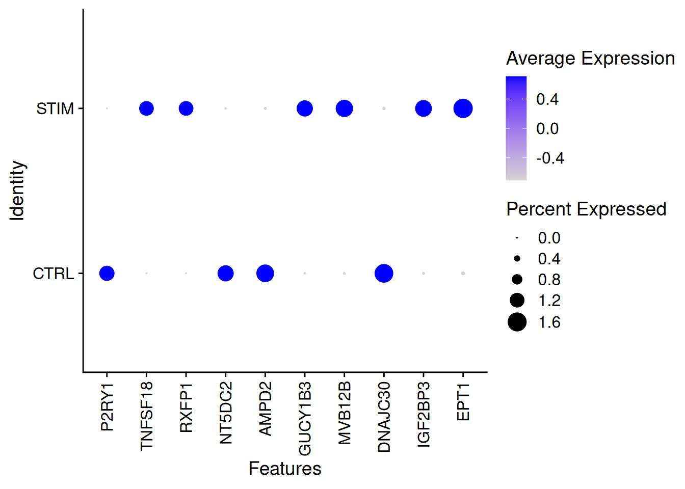
DotPlot(ifnb[,ICD14Mono],features=rownames(genetop_wilcox2)[1:10],
        group.by="donor.stim")+
  theme(axis.text.x = element_text(angle = 90, vjust = 0.5, hjust=1))
6.3.2 Test de DESeq2
pseudo_ifnb2 <- AggregateExpression(ifnb[,ICD14Mono],
                                   assays = "RNA",
                                   return.seurat = T,
                                   group.by = c("stim", "donor_id"))

cts2<-as.matrix(pseudo_ifnb2@assays$RNA$counts)
coldata2<-pseudo_ifnb2@meta.data
dds2 <- DESeqDataSetFromMatrix(countData = cts2,
                              colData = coldata2,
                              design= ~ donor_id + stim)
dds2 <- DESeq(dds2,fitType = c("local"))
resultsNames(dds2) # lists the coefficients
[1] "Intercept" "donor_id_SNG.1015_vs_SNG.101"
[3] "donor_id_SNG.1016_vs_SNG.101" "donor_id_SNG.1039_vs_SNG.101"
[5] "donor_id_SNG.107_vs_SNG.101" "donor_id_SNG.1244_vs_SNG.101"
[7] "donor_id_SNG.1256_vs_SNG.101" "donor_id_SNG.1488_vs_SNG.101"
[9] "stim_STIM_vs_CTRL" resDEseq2<-results(dds2,name="stim_STIM_vs_CTRL")
length(which(resDEseq2$padj<0.01)) / nrow(resDEseq2)[1] 0.1761901genetopDEseq2<-as.data.frame(resDEseq2) %>%
filter(padj<0.01)%>%
arrange(desc(abs(log2FoldChange)))%>%
top_n(100)Selecting by padjDotPlot(pseudo_ifnb2,features=rownames(genetopDEseq2)[1:10],group.by="stim")+
theme(axis.text.x = element_text(angle = 90, vjust = 0.5, hjust=1))Warning: Scaling data with a low number of groups may produce misleading
results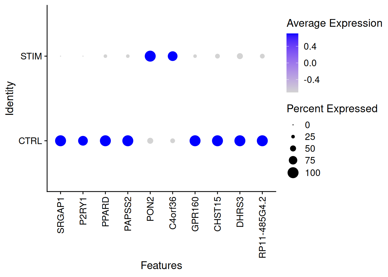
DotPlot(ifnb[,ICD14Mono],features=rownames(genetopDEseq2)[1:10],group.by="donor.stim")+
     theme(axis.text.x = element_text(angle = 90, vjust = 0.5, hjust=1))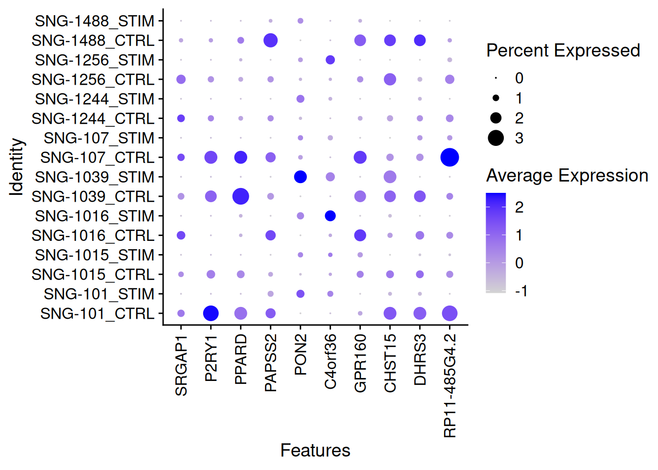
pheatmap(pseudo_ifnb2@assays$RNA$scale.data[rownames(genetopDEseq2),],
         cluster_cols = FALSE,
         scale = "column",
         show_rownames = FALSE,
         show_colnames = TRUE)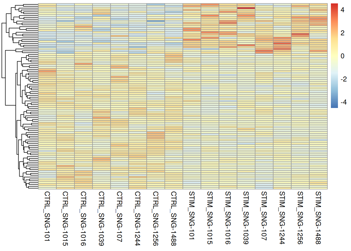
6.3.3 Test avec Nebula
Idents(ifnb)<-ifnb$seurat_annotations
ifnb_neb2<-scToNeb(obj=ifnb[,ICD14Mono],
                   assay="RNA",
                   id="donor_id",
                   pred=c("stim"))
df2 = model.matrix(~stim, data=ifnb_neb2$pred)
data_g2 = group_cell(count=ifnb_neb2$count,id=ifnb_neb2$id,pred=df2) # il faut grouper les cellules par indiv avant de faire nebula

#re2 = nebula(data_g2$count,data_g2$id,pred=data_g2$pred)
re2<-readRDS("Exercices/ResNebulaQ2.rds")

round(100*mean(p.adjust(re2$summary$p_stimSTIM,method="BH")<0.01),2)
[1] 47.75ifnbNebSumm2<-re2$summary
ifnbNebSumm2$padjStim<-p.adjust(re2$summary$p_stimSTIM,method="BH")
ifnbNebSumm2<-ifnbNebSumm2%>%
filter(padjStim <0.01)%>%
arrange(desc(abs(logFC_stimSTIM)))
head(ifnbNebSumm2) logFC_(Intercept) logFC_stimSTIM se_(Intercept) se_stimSTIM p_(Intercept)
1 -4.5536120 6.439125 0.51901138 1.00283914 1.730022e-18
2 0.6440147 6.390013 0.09225028 0.08222706 2.927358e-12
3 -0.8221986 6.099575 0.09229319 0.14361676 5.170400e-19
4 -3.7176773 5.960548 0.30092123 0.57837054 4.616411e-35
5 1.3395450 5.796196 0.05378646 0.05694309 6.588350e-137
6 -0.4725841 5.224608 0.07248106 0.09935159 7.025822e-11
p_stimSTIM gene_id gene padjStim
1 1.354757e-10 8963 CCNA1 7.830196e-10
2 0.000000e+00 10969 CCL8 0.000000e+00
3 0.000000e+00 3282 CXCL11 0.000000e+00
4 6.636461e-25 2620 HESX1 7.608229e-24
5 0.000000e+00 3281 CXCL10 0.000000e+00
6 0.000000e+00 7188 IFIT2 0.000000e+00genetopNeb2<-ifnbNebSumm2%>%
top_n(100)Selecting by padjStimDotPlot(ifnb[,ICD14Mono],features=genetopNeb2$gene[1:10],group.by="stim")+
theme(axis.text.x = element_text(angle = 90, vjust = 0.5, hjust=1))Warning: Scaling data with a low number of groups may produce misleading
results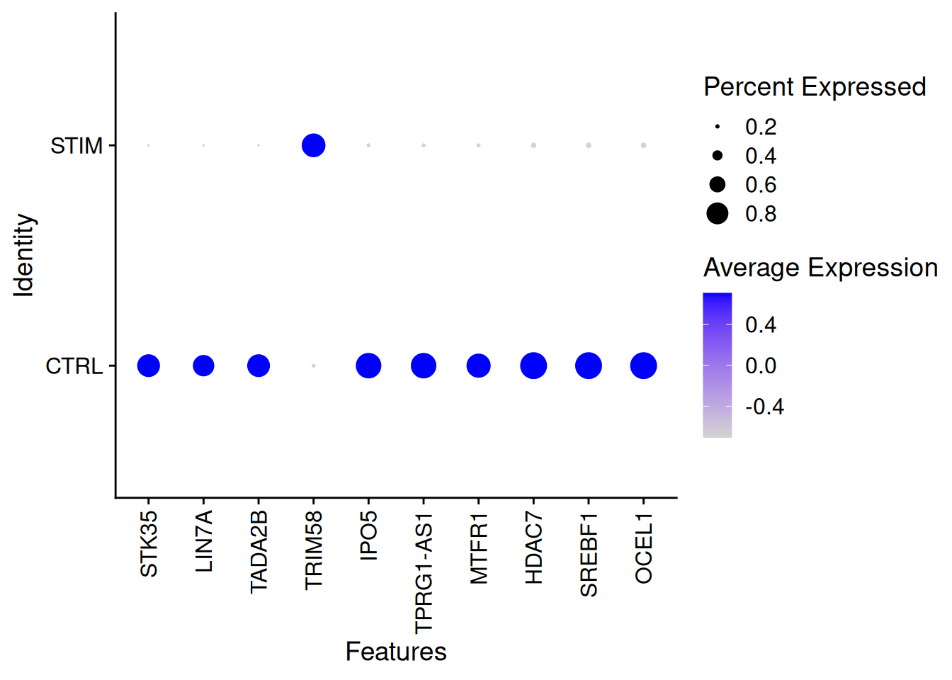
DotPlot(ifnb[,ICD14Mono],features=genetopNeb2$gene[1:10],group.by="donor.stim")+
  theme(axis.text.x = element_text(angle = 90, vjust = 0.5, hjust=1))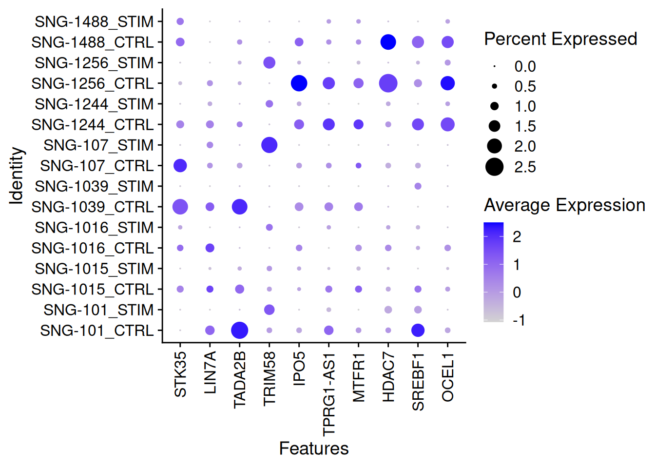
pheatmap(pseudo_ifnb2@assays$RNA$scale.data[genetopNeb2$gene,],
         cluster_cols = FALSE,
         scale = "row",
         show_rownames = FALSE,
         show_colnames = TRUE)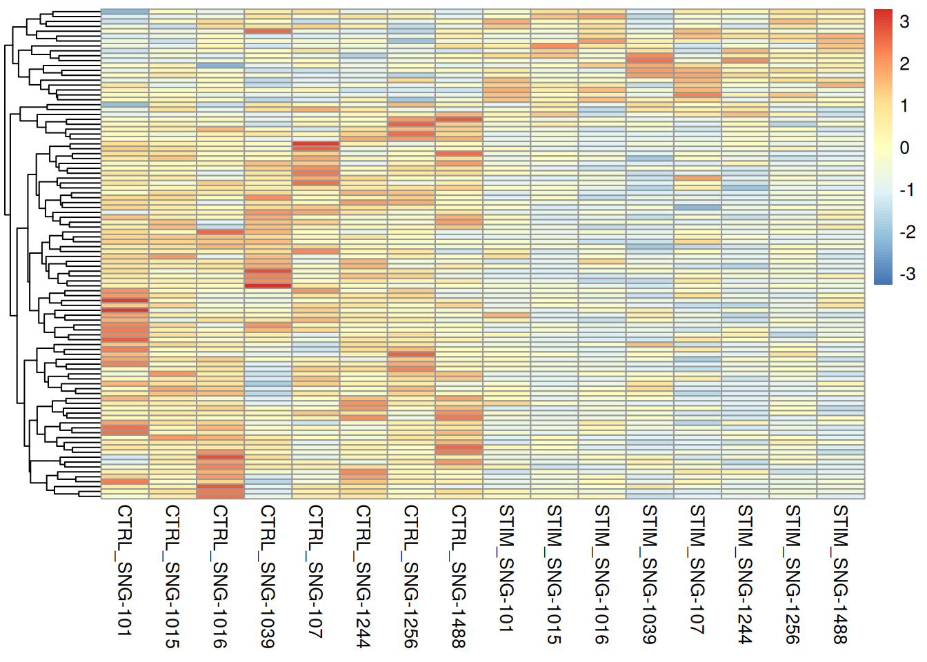
6.3.4 Par une approche supervisée (ex: Random Forest)
- Random Forest pour prédire STIM / CTRL
datatrain<-t(as.matrix(ifnb@assays$RNA$scale.data[,ICD14Mono]))
dataRF<-data.frame(datatrain,
                   Cl = as.factor(ifnb$stim[ICD14Mono]))

#resRF<-randomForest(Cl ~ ., data = dataRF,importance=T,proximity=T)
resRF<-readRDS("Exercices/resNF.rds")

table(resRF$predicted,dataRF$Cl)
       CTRL STIM
  CTRL 2158    1
STIM 9 2085- Importance des variables
p1<-ggvip(resRF,num_var = 20,type=1)
p2<-ggvip(resRF,num_var = 20,type=2)

p1$vip + p2$vip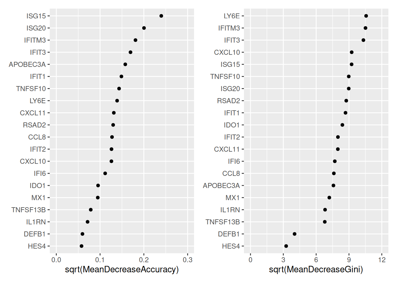
genetopRF2<-as.data.frame(resRF$importance)%>%
      arrange(desc(MeanDecreaseGini))%>%
      top_n(100)
Selecting by MeanDecreaseGiniDotPlot(ifnb[,ICD14Mono],features=rownames(genetopRF2)[1:10],group.by="stim")+
theme(axis.text.x = element_text(angle = 90, vjust = 0.5, hjust=1))Warning: Scaling data with a low number of groups may produce misleading
results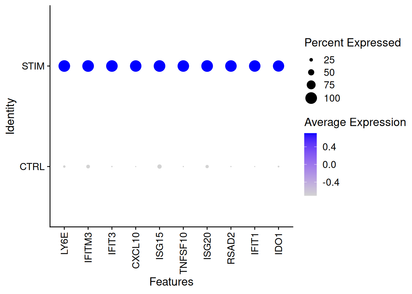
DotPlot(ifnb[,ICD14Mono],features=rownames(genetopRF2)[1:10],group.by="donor.stim")+
  theme(axis.text.x = element_text(angle = 90, vjust = 0.5, hjust=1))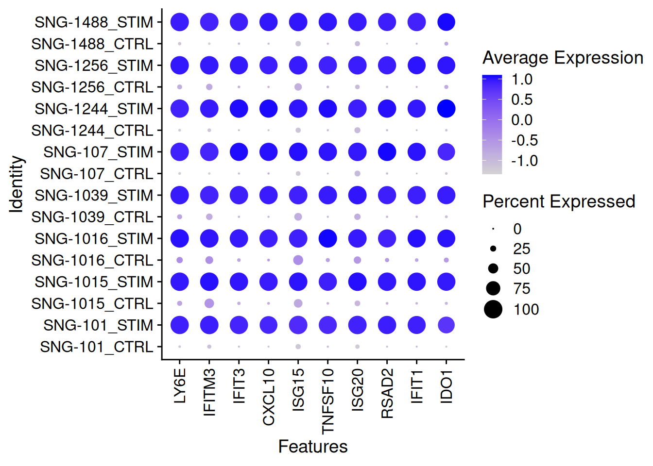
II<-which(rownames(pseudo_ifnb2@assays$RNA$scale.data) %in% rownames(genetopRF2))
pheatmap(pseudo_ifnb2@assays$RNA$scale.data[II,],
         cluster_cols = FALSE,
         scale = "row",
         show_rownames = FALSE,
         show_colnames = TRUE)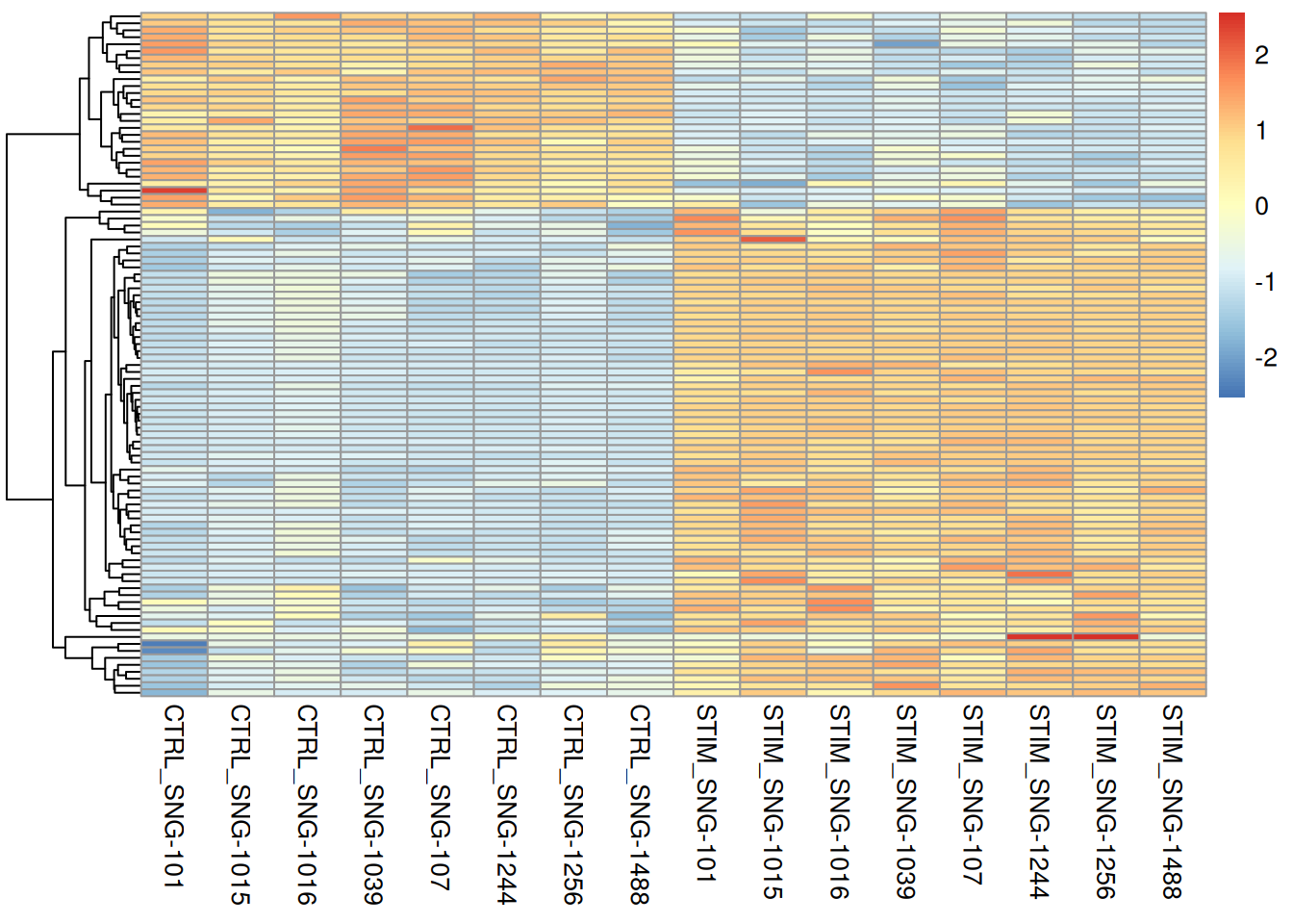
6.3.5 Comparaison
ggvenn(list(DEseq2=rownames(genetopDEseq2),
            Nebula=genetopNeb2$gene,
            Wilcox=rownames(genetop_wilcox2),
            RF=rownames(genetopRF2)))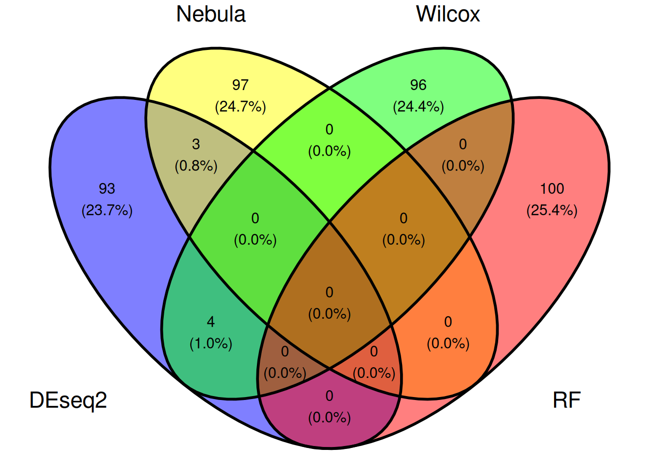
7 Analyse fonctionnelle des gènes
7.1 Choix de la liste de gènes à analyser
- Question 1 : déterminer les gènes dont l’expression varie entre les deux conditions (types cellulaires confondus) :
- Test de Wilcoxon :
res1_Wilcox - Avec DESeq2 dans
FindMarkers:bulk.cond1 - DESeq2 :
resDEseq1 - NEBULA :
ifnbNebSumm1
- Test de Wilcoxon :
- Question2 : déterminer les gènes dont l’expression varie entre les deux conditions pour le type cellulaire “CD14 Mono” fixé :
- Test de Wilcoxon :
res2_Wilcox - Avec DESeq2 dans
FindMarkers:bulk.cond2 - DESeq2 :
resDEseq2 - NEBULA :
ifnbNebSumm2
- Test de Wilcoxon :
On choisi les gènes différentiellement exprimés avec méthode DESeq2 de Seurat pour la Question 1 :
genes <- bulk.cond1  |> filter(p_val_adj<0.01)  |> rownames()
genes
[1] "NT5C3A" "IFI16" "ISG20" "DDX58"
[5] "RTP4" "TRIM22" "C19orf66" "PPM1K"
[9] "SP110" "IL1RN" "TREX1" "PHF11"
[13] "HERC5" "SAMD9" "CCL8" "DHX58"
[17] "MT2A" "IDO1" "HSH2D" "SOCS1"
[21] "IFITM2" "EIF2AK2" "PARP9" "XRN1"
[25] "IFITM1" "IFIT5" "RBCK1" "NEXN"
[29] "RABGAP1L" "CD164" "HES4" "NMI"
[33] "HERC6" "SPATS2L" "NCOA7" "PNPT1"
[37] "CXCL11" "PSMA2.1" "SP100" "IFIH1"
[41] "TRADD" "DDX60" "NUB1" "IFI35"
[45] "HELZ2" "PARP14" "IRF7" "DRAP1"
[49] "TMEM140" "IRF2" "RNF213" "SLC38A5"
[53] "TMSB10" "STAT1" "PARP12" "C5orf56"
[57] "MX2" "SLAMF7" "SSB" "BAG1"
[61] "TMEM123" "CXCL10" "TNFSF10" "PARP10"
[65] "HAPLN3" "IFIT2" "FAM46A" "ZBP1"
[69] "SAMD9L" "CFLAR" "IFIT3" "GBP4"
[73] "CHST12" "OAS1" "CMPK2" "ADAR"
[77] "FBXO6" "DCK" "TRAFD1" "SP140"
[81] "ELF1" "RTCB" "GCH1" "TRIM14"
[85] "IRF8" "EPSTI1" "DTX3L" "UBE2L6"
[89] "PARP11" "OASL" "ISG15" "DDX60L"
[93] "SMCHD1" "USP15" "DYNLT1" "IL27"
[97] "BST2" "VCAN" "PSMA4" "BLZF1"
[101] "LY6E" "CD38" "STAT2" "STOM"
[105] "HSPA1A" "TNFSF13B" "NAPA" "MOV10"
[109] "GMPR" "HESX1" "APOL3" "OPTN"
[113] "IL15RA" "PLSCR1" "SAMD4A" "OAS3"
[117] "CNP" "APOL6" "XAF1" "TRIM5"
[121] "GSDMD" "IFIT1" "GPBP1" "MX1"
[125] "TAP1" "KIAA0040" "PI4K2B" "PML"
[129] "KPNB1" "NADK" "GBP1" "CHMP5"
[133] "TARBP1" "ZNFX1" "OAS2" "FAS"
[137] "SNX6" "AIM2" "IRF9" "CD47"
[141] "HLA-E" "TRIM21" "RSAD2" "ODF2L"
[145] "WARS" "PRR5" "TAPBP" "USP30-AS1"
[149] "LGALS9" "PCGF5" "PPP2R2A" "BBX"
[153] "PSMA5" "CLEC5A" "LTA4H" "LMNB1"
[157] "PSMB9" "NDUFA9" "DECR1" "IFI44"
[161] "INSIG1" "TMX1" "CTD-2521M24.9" "IRG1"
[165] "MDK" "ADPRHL2" "BLVRA" "CD274"
[169] "LAMP3" "C1GALT1" "PSMB8" "CXorf21"
[173] "TAP2.1" "MARCKS" "NBN" "MMP9"
[177] "TRIM38" "CD40" "SP140L" "DEFB1"
[181] "BAZ1A" "LYSMD2" "IL8" "NUPR1"
[185] "HSPB1" "APOBEC3A" "GLIPR1" "MYL12A"
[189] "BRK1" "CASP10" "N4BP1" "IL4I1"
[193] "MTHFD2" "CD14" "DUSP5" "BCL2L14"
[197] "WIPF1" "CASP8" "NUCB1" "TDRD7"
[201] "MB21D1" "OGFR" "IFI6" "TGM1"
[205] "GBP2" "ARL6IP6" "RNF114" "MAX"
[209] "GNB4" "CBWD2" "ARL5B" "CD48"
[213] "CCNA1" "GBP3" "IQGAP2" "CBR1"
[217] "TRAM1" "SIGLEC1" "PSME2" "TMEM110"
[221] "IFITM3" "B2M" "SAT1" "LAG3"
[225] "HSP90AA1" "PRKD2" "RBM7" "PGAP1"
[229] "LPIN2" "SUB1" "RP11-701P16.5" "RAB8A"
[233] "TRANK1" "DENND1B" "TBXAS1" "LAP3"
[237] "JUP" "CLEC2B" "SGTB" "SAP18"
[241] "ZC3HAV1" "AMICA1" "PRDX4" "DNAJA1"
[245] "RARRES3" "ACOT9" "CNDP2" "UNC93B1"
[249] "PID1" "CD80" "MASTL" "IGFBP4"
[253] "TXN" "DNPEP" "CXCL9" "DAPP1"
[257] "VAMP5" "MKRN1" "CAST" "PDGFRL"
[261] "C1GALT1C1" "FOS" "TMEM50A" "ETV7"
[265] "FAM72B" "FBXO7" "SCIN" "DEK"
[269] "S100A8" "TBC1D1" "IL1B" "RAD9A"
[273] "MNDA" "CMKLR1" "RIN2" "GCNT2"
[277] "CH25H" "KLF6" "ATP2B1" "ATG3"
[281] "GTF2B" "CYP27A1" "MIA3" "GCA"
[285] "GPR141" "ARHGEF3" "CD69" "SPTLC2"
[289] "BATF2" "EIF3L" "EXOC3L1" "APOL1"
[293] "ANKRD22" "QPCT" "ATF3" "ICAM2"
[297] "CIR1" "C3orf38" "C19orf59" "SNX10"
[301] "MYCBP2" "IL13RA1" "C4orf3" "SRGAP2"
[305] "SNN" "HSP90AB1" "B3GNT2" "TOR1B"
[309] "MLKL" "CASP4" "SLC31A2" "LYN"
[313] "SORL1" "NAGK" "CD2AP" "KARS"
[317] "TINF2" "ATF5" "SPSB1" "PRF1"
[321] "TMEM60" "PMAIP1" "MCL1" "MVP"
[325] "TFG" "FYTTD1" "TAGAP" "ARHGAP25"
[329] "FERMT3" "ATP5F1" "GALM" "HELB"
[333] "SNX2" "IFI44L" "HSPA8" "ARL8B"
[337] "TFEC" "TRIM69" "FAM8A1" "PLAC8"
[341] "ADAM19" "GTF2E2" "NT5C2" "SFT2D2"
[345] "CMC2" "LILRA5" "SAMHD1" "RNF138"
[349] "APOBEC3F" "TMEM126B" "EHD4" "TANK"
[353] "RRBP1" "RP11-343N15.5" "FUT4" "CLTB"
[357] "HRASLS2" "DRAM1" "ACTA2" "ENDOD1"
[361] "CASP7" "AIDA" "SLC25A28" "SERPING1"
[365] "CLIC2" "RIN3" "FAM26F" "SLC7A11"
[369] "PRLR" "HBEGF" "CCR5" "GIMAP4"
[373] "DOCK8" "RASGRP3" "TIA1" "NUDCD1"
[377] "CXXC5" "PLXDC2" "CD53" "SYNE2"
[381] "HEXDC" "OSM" "GPR180" "TNFAIP6"
[385] "TKT" "MTSS1" "MRPL17" "PIK3AP1"
[389] "TPST1" "CDKN2D" "STX17" "CST6"
[393] "IL15" "PLIN2" "GNG5" "POLR2E"
[397] "HERPUD2" "CALCOCO2" "STAP1" "CTSZ"
[401] "RGCC" "TLR7" "YBX1" "CLEC2D"
[405] "HNMT" "DNAJB4" "CAMK1" "RIPK2"
[409] "SHISA5" "IRF1" "ZNHIT1" "CASP3"
[413] "CKB" "SOBP" "FAM72A" "UBE2F"
[417] "FAM50A" "CTD-2037K23.2" "CXorf38" "PSME1"
[421] "SCARB2" "UBXN2A" "OSBPL1A" "MCOLN2"
[425] "MSR1" "RP11-445H22.3" "EXOSC9" "ORAI3"
[429] "DERL1" "SCLT1" "NCF1" "CASP1"
[433] "ARID5A" "PLEK" "ITM2B" "GPR171"
[437] "RNASEH2B" "DAB2" "STX11" "BAK1"
[441] "CLIC4" "MAT2B" "GOLGA4" "UBE2Z"
[445] "CACNA1A" "SDC2" "MYD88" "PARP8"
[449] "THBD" "BRCA2" "CHRNB1" "HDAC1"
[453] "TWF2" "CSRNP1" "ST3GAL5" "YPEL3"
[457] "JAK2" "MORC3" "EDEM1" "TCF4"
[461] "PELI1" "NASP" "UBE2D3" "ATP6V1H"
[465] "RP11-420G6.4" "MSL3" "CMTR1" "USP18"
[469] "UBA7" "ARL6IP4" "RPS6KA1" "TYMP"
[473] "GATSL3" "LMO2" "APOBEC3G" "MLTK"
[477] "AC007036.6" "ZFP36L1" "GADD45B" "TPI1"
[481] "TRIM25" "NINJ1" "PRKX" "DNAAF1"
[485] "ENG" "AC004988.1" "NUMB" "CUL1"
[489] "CDS2" "PPA1" "C9orf72" "IER3"
[493] "PIM3" "ARHGAP18" "CATSPER1" "PAPD7"
[497] "IRGQ" "PTPLAD2" "TUBA4A" "ABCC3"
[501] "PTGS1" "AP5B1" "SLFN12" "CTB-61M7.2"
[505] "CFB" "QSOX1" "UTRN" "GPR155"
[509] "FFAR2" "TRIM56" "RBM43" "PANK2"
[513] "APPL1" "ID3" "GIMAP2" "KCNJ15"
[517] "UQCRB" "ANKFY1" "RDH14" "LYPD2"
[521] "DCP1A" "POLD4" "C21orf91" "FAR2"
[525] "GCNT1" "AHSA1" "KCNA3" "CYP2J2"
[529] "CTD-2336O2.1" "MESDC2" "WDFY1" "SCPEP1"
[533] "SRSF9" "ATXN1" "CD9" "AC009948.5"
[537] "RP11-288L9.1" "HAVCR2" "PHACTR4" "CCRL2"
[541] "HTRA1" "JARID2" "NR4A3" "UBAC1"
[545] "HBP1" "KCNN4" "PANX1" "EXT1"
[549] "FKBP11" "SLC25A11" "STAT3" "PCMT1"
[553] "SMOX" "SPN" "RAB4A" "GBP5"
[557] "MRPS18C" "TNK2" "BRIP1" "NDFIP1"
[561] "UBQLN2" "SERPINB1" "EDN1" "CCL4"
[565] "PABPC4" "CARD16" "OSBPL9" "GPX1"
[569] "SMPDL3A" "CCDC85B" "TRIM44" "HIPK2"
[573] "MAP1LC3A" "AP2S1" "CXCL1" "C4orf32"
[577] "RPS6KB2" "TPMT" "CALM1" "LGALS3BP"
[581] "OAZ2" "ZCCHC2" "RRAGC" "BATF3"
[585] "SLC18B1" "GLRX" "TRIM26" "MARCKSL1"
[589] "LIPA" "PHLDA1" "PKD2L1" "MS4A6A"
[593] "RAB7L1" "H3F3B" "RP11-326I11.3" "RPS6KA5"
[597] "RAB31" "FOXN2" "BARD1" "CD82"
[601] "FGD2" "FARP1" "SH3GLB1" "LILRB1"
[605] "GPD2" "GTPBP1" "RFX2" "RBMS1"
[609] "DESI1" "PDCD6" "STK24" "CCDC50"
[613] "KIAA0226" "AC093673.5" "KIFC3" "ST14"
[617] "NMB" "GBP7" "CYTH4" "TPST2"
[621] "JTB" "PPARG" "GRIN3A" "VCPIP1"
[625] "TMEM14C" "TXNIP" "EMC2" "SETX"
[629] "MICB" "MEF2A" "RP11-274B18.2" "HIP1"
[633] "RGL1" "PDLIM7" "ADAMDEC1" "HINT3"
[637] "DLAT" "SLC38A6" "CYLD" "MOB3C"
[641] "GMDS" "PRDX5" "TNFSF18" "CNPPD1"
[645] "CAPN2" "BLNK" "SDHA" "WDR41"
[649] "AC010226.4" "ARHGAP27" "EXOC2" "PPM1M"
[653] "SCIMP" "RBX1" "EEPD1" "PGD"
[657] "CNPY3" "SNX3" "PDCD1LG2" "CKS1B"
[661] "WBP1L" "C9orf91" "ATP10A" "FAM177A1"
[665] "PAIP1" "C14orf159" "CECR1" "MIER1"
[669] "TPM3" "ARAP2" "TMEM229B" "MRPL32"
[673] "RAB8B" "SIVA1" "FXYD6" "STK38L"
[677] "EXOSC4" "DDX5" "CTSA" "MIR142"
[681] "SECTM1" "RNF19B" "C17orf67" "OSBPL8"
[685] "RP11-65J3.1" "FKBP5" "NECAP2" "BCKDK"
[689] "RBMS2" "FAM122C" "RAPGEF2" "MAGT1"
[693] "SRSF5" "YWHAQ" "SRP54" "ARRDC2"
[697] "FAM19A2" "AP000640.2" "IGSF6" "CD163"
[701] "ASL" "SPG20" "CD93" "CKAP4"
[705] "HIAT1" "PATL2" "ZNF277" "ADPRH"
[709] "CCSER2" "MOB1A" "DKFZP761J1410" "CBWD5"
[713] "TMEM187" "C11orf31" "CITED2" "EIF4E3"
[717] "HLA-A" "PNPLA6" "TBC1D7" "TNFSF14"
[721] "CD44" "PKM" "IKBKE" "RAD23A"
[725] "SEC62" "SSTR2" "GSTP1" "EPB41L3"
[729] "MKKS" "GNA15" "CTSS" "UBC"
[733] "SLC25A3" "CTNNBIP1" "PHACTR2" "KLF5"
[737] "ATP13A3" "RILPL2" "BAD" "THBS1"
[741] "GAPT" "ZMIZ1" "NLRC4" "CCR1"
[745] "AKAP7" "ENPP2" "KCNAB2" "AC009133.12"
[749] "LMO4" "HLA-F" "RIPK1" "SLC35A5"
[753] "RP1-197B17.3" "GIMAP6" "CTNNBL1" "PLEK2"
[757] "BCAT1" "SPG21" "SIRT2" "RALB"
[761] "HM13" "CLEC4A" "B4GALT5" "ITGAE"
[765] "NLRC5" "SLC27A3" "EEF1A1" "TNFAIP8L1"
[769] "GRIPAP1" "RPL6" "SLC25A39" "IDS"
[773] "SAT2" "CORO1B" "TM6SF1" "FAM89B"
[777] "IDO2" "EIF3D" "GNAI3" "HSPA1B"
[781] "CDC73" "HNRNPDL" "RXFP1" "ASCL2"
[785] "ATP1A1" "MR1" "LRP1" "KCTD14"
[789] "H2AFY" "MAD2L1BP" "PLAU" "BTG3"
[793] "GIMAP8" "PSTPIP1" "ACTN1" "PPIF"
[797] "ETNK1" "DOK3" "EMD" "FRMD3"
[801] "ERO1L" "AZI2" "MED25" "MORF4L1"
[805] "N4BP2L1" "LINC00158" "POMP" "NABP1"
[809] "ATP6AP1" "RAB34" "NUP214" "GUCY1A3"
[813] "RP11-408H1.3" "CHORDC1" "TAX1BP3" "UQCRC1"
[817] "PSMA3" "NHLRC3" "VEGFA" "UFD1L"
[821] "TMEM219" "MAP2K6" "SRSF4" "ANKIB1"
[825] "MEFV" "LNPEP" "TCN2" "CNIH4"
[829] "NISCH" "HIST1H2AC" "HNRNPM" "GGA1"
[833] "MCOLN1" "ABCD1" "ALCAM" "ARL3"
[837] "PSMG2" "PLEKHF2" "ARHGDIB" "APOL2"
[841] "C18orf25" "ERCC1" "AXL" "EMC3"
[845] "AAED1" "OTOF" "CGGBP1" "PSMB10"
[849] "UTP11L" "GLIS3" "ARMCX1" "VNN1"
[853] "PARP4" "HNRNPF" "RASSF4" "CR1L"
[857] "PARP15" "TMEM19" "AGO1" "TSPAN13"
[861] "S100A2" "GSTK1" "CXCL5" "ITGB1"
[865] "HIST2H2BE" "RNF19A" "SMARCA5" "CTSC"
[869] "GOLM1" "UBE2D1" "IER2" "EMP1"
[873] "SLC25A5" "TMEM170A" "SSU72" "BCL11A"
[877] "SLC16A6" "LILRB2" "BEST1" "P2RY6"
[881] "RERE" "GZMB" "SDS" "ACSL1"
[885] "ARF5" "LINC00984" "KDSR" "NEDD1"
[889] "SLC11A1" "RASGEF1B" "GPR108" "RNF130"
[893] "TOP1" "CXCL13" "GTPBP2" "SERPINB9"
[897] "ESD" "CCND2" "MMP14" "FAM43A"
[901] "SLC41A2" "RNASE2" "RP11-737O24.1" "COL7A1"
[905] "SCT" "BBC3" "AKR7A2" "MRPL44"
[909] "SLC16A10" "HCLS1" "RPA3" "L3HYPDH"
[913] "ALPK1" "CTSH" "ZNF620" "BCL2L13"
[917] "BLMH" "H2AFV" "PDE7A" "NDUFB10"
[921] "SLC25A6" "PFN1" "SQRDL" "GIMAP7"
[925] "FAM111A" "HLA-C" "CD1D" "HAX1"
[929] "ST8SIA4" "RBMX" "CLDND1" "ACTB"
[933] "LILRB4" "GNA12" "SIGLEC9" "UBE2S"
[937] "RBBP6" "RPS19BP1" "TLR4" "FCAR"
[941] "ARID4B" "WHSC1L1" "FNIP2" "BTN3A1"
[945] "SH3BP5" "GLIPR2" "PAPSS2" "NLN"
[949] "DOK2" "ANXA1" "RNF168" "NFE2L3"
[953] "CCS" "C7orf49" "ARL6IP5" "APH1B"
[957] "FTH1" "PKIB" "XIAP" "RAB3GAP1"
[961] "RABGGTA" "STAB1" "IL16" "KCTD20"
[965] "NCKAP1L" "CEBPA" "RP11-532F6.3" "STRA13"
[969] "EVI5" "CD101" "ZNF106" "IPCEF1"
[973] "MOB3A" "RBM11" "PLXND1" "SAYSD1"
[977] "RP11-480C16.1" "TALDO1" "E2F5" "SELL"
[981] "CDC42EP1" "YEATS2" "TNFRSF12A" "SMPD3"
[985] "LINC00926" "JADE2" "FGL2" "TMEM167A"
[989] "CNTRL" "EFR3A" "CCL7" "AQP9"
[993] "PDE4B" "NDUFA2" "ANXA4" "PARK7"
[997] "SLC37A1" "DPEP2" "CORO1A" "TANC2"
[1001] "HP1BP3" "CTNND1" "PIK3R5" "SLC35A4"
[1005] "SYNJ2BP" "SSR4" "KAT2A" "STX18"
[1009] "RNF7" "ATP6V0B" "RICTOR" "MAPK1"
[1013] "RP11-10J5.1" "C10orf54" "ZRSR2" "COTL1"
[1017] "PRPS2" "ZBTB43" "FANCA" "CAPZB"
[1021] "MS4A7" "TMEM251" "GALNT1" "IFI27"
[1025] "EHD1" "SMC6" "ATL3" "PREX1"
[1029] "ABHD8" "HNRNPA1" "DEDD2" "CREG1"
[1033] "RBM14" "UBE2B" "RP2" "USP33"
[1037] "RP11-63P12.6" "PTGFRN" "HDGF" "SCO2"
[1041] "COMMD3" "MITF" foldChange <- bulk.cond1|> filter(p_val_adj<0.01) |> pull(avg_log2FC)
names(foldChange) <- genesLes gènes sont identifiés selon leur nom ou “gene symbol”. Pour obtenir la meilleure correspondance possible avec les bases de données, on va les convertir en entrez id, qui sont les identifiants de la base de données gene du ncbi :
eg = clusterProfiler::bitr(genes, fromType="SYMBOL", toType="ENTREZID", OrgDb="org.Hs.eg.db")'select()' returned 1:1 mapping between keys and columnsWarning in clusterProfiler::bitr(genes, fromType = "SYMBOL", toType =
"ENTREZID", : 8.06% of input gene IDs are fail to map...eg |> as_tibble() |> rmarkdown::paged_table()Il existe d’autres identifiants et d’autres méthodes pour convertir les identifiants, comme la librairie R biomaRt et les identifiants ensembl :
require(biomaRt)
ensembl <- useEnsembl(biomart = "ensembl", dataset = "hsapiens_gene_ensembl",version =114)


gene_conversion <- getBM(attributes = c("ensembl_gene_id","entrezgene_id","hgnc_symbol"),
      filters = "hgnc_symbol",
      values = genes,
      mart = ensembl)
gene_conversion %>% as_tibble() %>% rmarkdown::paged_table()
7.2 Les outils d’analyse d’enrichissement
7.2.1 Outils en ligne
7.2.2 Packages R
ClusterProfilerhypeRgprofiler2fgsea(utilisé en interne par ClusterProfiler)
Dans ce TP nous utiliserons uniquement ClusterProfiler car il est très complet et bien documenté (voir ici et ici)
7.3 Différentes sources de voies biologiques
- Gene Ontology (GO)
- KEGG (Kyoto Encyclopedia of Genes and Genomes)
- WikiPathways
- Disease Ontology
- Reactome
- MSigDB (Molecular Signatures Database)
- MeSH (Medical Subject Headings)
Dans ce TP nous utiliserons uniquement la Gene Ontology, mais c’est possible d’utiliser les autres avec ClusterProfiler
7.3.1 Gene Ontology (GO)
7.3.2 Site web : http://geneontology.org/
7.3.3 Description :
GO est une base de données très utilisée qui classe les gènes selon trois grandes ontologies :
- Molecular Function
- Activités élémentaires d’un produit génique au niveau moléculaire.
- Biological Process
- Suite coordonnée d’événements impliquant plusieurs fonctions moléculaires.
- Cellular Component
- Structures ou localisations cellulaires où les produits géniques sont actifs.
7.4 Approches d’enrichissements
Analyse de Surreprésentation (ORA - Over Representation Analysis) : Cette méthode détermine si les gènes différentiellement exprimés sont enrichis dans des voies spécifiques ou des groupes ontologiques.
Analyse d’Enrichissement de Groupes de Gènes (GSEA - Gene Set Enrichment Analysis) : GSEA évalue si un ensemble pré-défini de gènes présente des différences statistiquement significatives entre deux ou plusieurs conditions biologiques.
Dans ClusterProfiler, les fonctions gseGO() et enrichGO permettent d’utiliser ces deux méthodes avec la Gene Ontology
7.5 Enrichissement par analyse de sur-représentation (ORA - Over Representation Analysis)
L’Analyse de Surreprésentation (ORA) est une méthode courante pour identifier si certaines fonctions ou processus biologiques connus sont surreprésentés (= enrichis) dans une liste de gènes obtenue expérimentalement


7.6 Analyse GO de sur-représentation avec R et clusterProfiler
On utilise enrichGO() sur nos gènes différentiellement exprimés (objet eg).
org.db <- org.Hs.eg.db::org.Hs.eg.db
ego <- enrichGO(gene = eg$ENTREZID,
universe = NULL,
OrgDb = org.db,
keyType = "ENTREZID",
ont = "BP",
pAdjustMethod = "BH",
pvalueCutoff = 0.05,
qvalueCutoff = 0.05,
readable = TRUE)
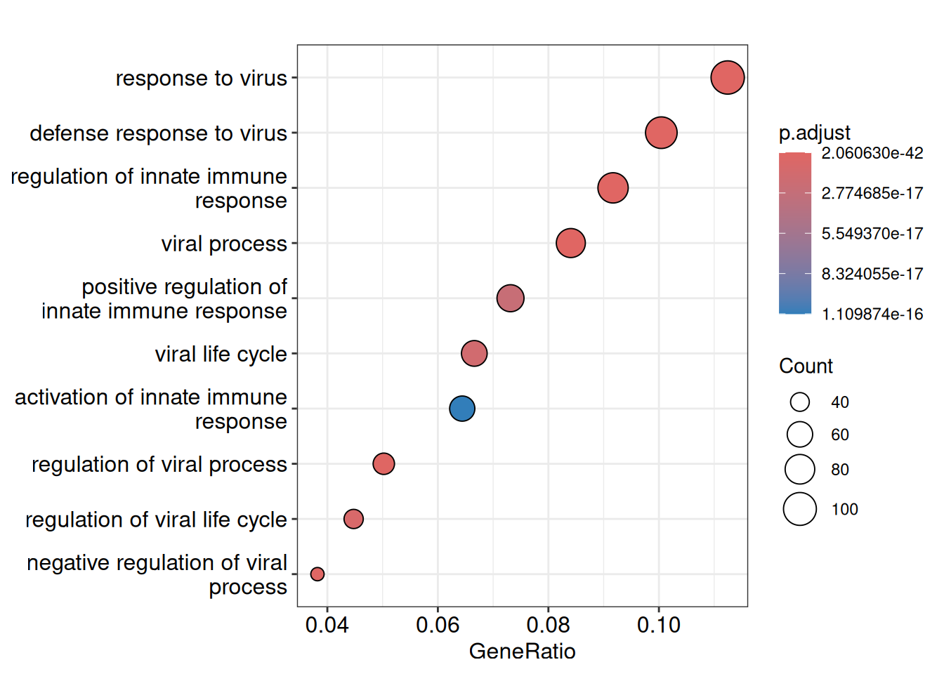
ego |> as_tibble() |> rmarkdown::paged_table()7.6.1 Méthodes de visualisation des résultats d’enrichissement
Voir ici pour la liste complète
7.6.1.1 Dotplot
7.6.1.2 Gene-Concept Network
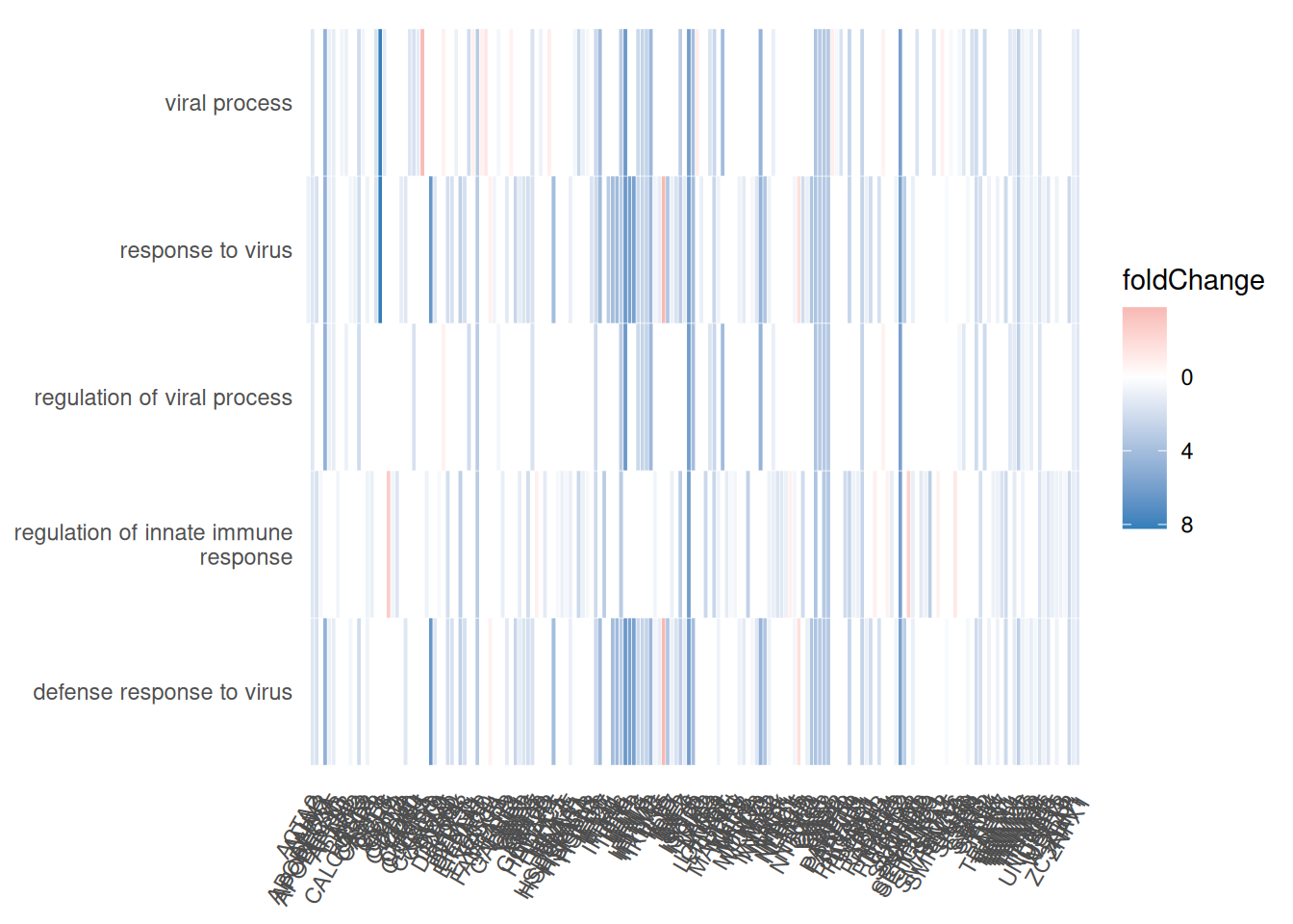
Récupérer la valeur du fold-change :
foldChange <- foldChange |> enframe() |> left_join(eg,by = c("name"="SYMBOL")) |> dplyr::select(ENTREZID,value) |> drop_na() |> deframe()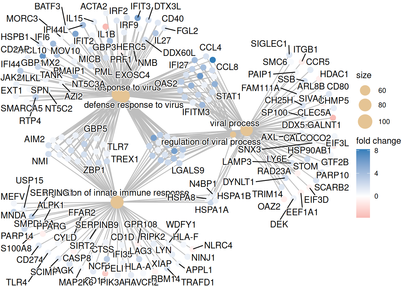
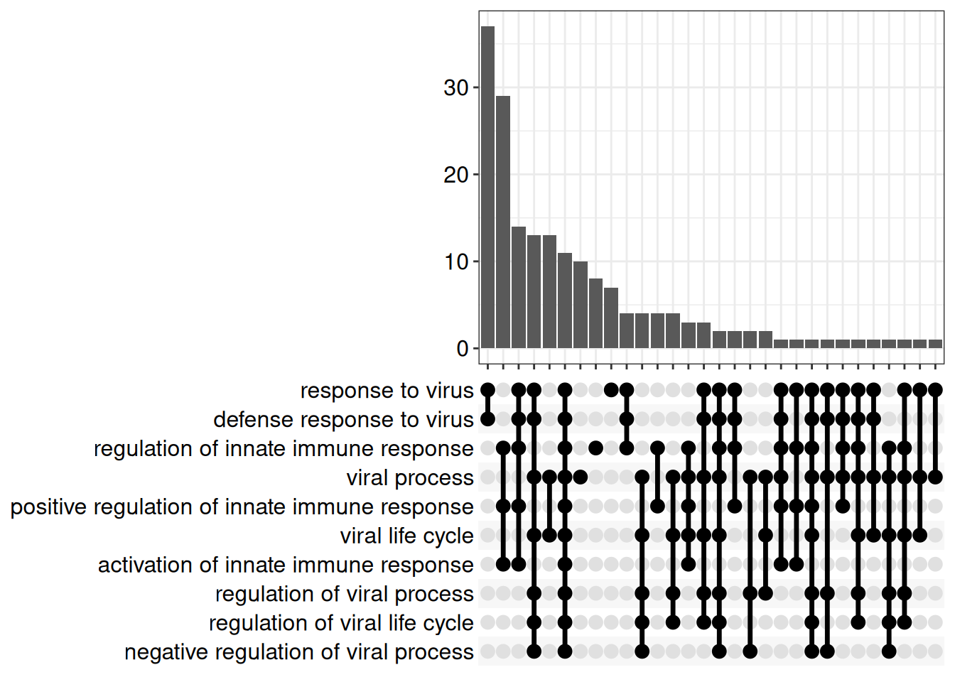
7.6.1.3 UpSet plots
7.6.1.4 Gene-Concept Network