Initiation à l’analyse
de données single-cell RNA-seq
avec Seurat

Cours

Cathy Maugis-Rabusseau & Vincent Rocher

Introduction

What is single-cell RNA-seq data?

Principle of bulk RNA-seq

bulkRNAseq

Principle of single-cell RNA-seq (scRNA-seq)

scRNAseq

From Sample Preparation to Bioinformatics

Different Technologies

From (Baysoy et al. 2023)

From Sample Preparation to Bioinformatics

Alignment & Filtering

• After sample preparation, the process moves to bioinformatics
• Sequence alignment, selection of usable cells, etc.

With CellRanger

From Sample Preparation to Bioinformatics

Algorithm of CellRanger

Key steps:

• Read trimming
• Demultiplexing & UMI storage
• Alignment
• UMI counting

UMI counting

From Sample Preparation to Bioinformatics

Output from CellRanger

Output from CellRanger

From Sample Preparation to Bioinformatics

Other Tools

• The Salmon suite for single-cell: alevin
• UMI processing with a standard pipeline: umi-tools

Other Pipelines

• scrnaseq from nf-core

From Sample Preparation to Bioinformatics

After the Bioinformatics Step

For 10X Data

Read10X Reference

• 3 files: features, barcodes, and count matrix (matrix.mtx)

Read10X(
  data.dir,
  gene.column = 2,
  cell.column = 1,
  unique.features = TRUE,
  strip.suffix = FALSE
)

For alevin

• quants_mat.gz – Compressed count matrix.
• quants_mat_cols.txt – Column Header (Gene-ids) of the matrix.
• quants_mat_rows.txt – Row Index (CB-ids) of the matrix.
• quants_tier_mat.gz – Tier categorization of the matrix.

quants_tier_mat.gz

• Tier 1 is the set of genes where all the reads are uniquely mapping.
• Tier 2 is genes that have ambiguously mapping reads, but connected to unique read evidence as well, that can be used by the EM to resolve the multimapping reads.
• Tier 3 is the genes that have no unique evidence and the read counts are, therefore, distributed between these genes according to an uninformative prior.

# Reading in the alevin quants quants using tximport
txi <- tximport(files, type="alevin")

From the biological questions to the statistical questions

Biological questions

• Are there distinct subpopulations of cells?
• For each cell type, what are the marker genes?
• How visualize the cells?
• Are there continuums of differentiation / activation cell states?
• …

(Rostom et al. 2017)

From the biological questions to the statistical questions

Statistical analysis

• Clustering of cells
• Variable (gene) selection in learning or differential analysis (hypothesis testing)
• Reduction dimension
• Network inference
• Pseudo-time inference
• …

(Rostom et al. 2017)

Packages to analyze scRNA-seq data

Number of available tools for scRNA-seq data

• Many packages are released regularly for scRNA-seq data analysis.
• You can follow the news in the “Updates” section of scRNA-tools.

Packages to analyze scRNA-seq data

Some bioinfo-stat pipelines/workflows

• Seurat
• SCANPY
• Sincell
• simpleSingleCell
• SINCERA
• Scedar

• R package Seurat V5
• Its own object \(\longrightarrow\) Seurat Object

• References: (Hao et al. 2023, 2021; Stuart et al. 2019; Butler et al. 2018; Satija et al. 2015)

• Python package SCANPY
• Its own object \(\longrightarrow\) AnnData class

• References: (Wolf, Angerer, and Theis 2018)

• R package Sincell
• Its own object \(\longrightarrow\) Sincell Object

• References: (Juliá, Telenti, and Rausell 2015)

• R package simpleSingleCell

• References: (Lun, McCarthy, and Marioni 2016)

• R package SINCERA

• References: (Guo et al. 2015)

• Python package Scedar

• References: (Zhang et al. 2020)

Data used for presentation / exercices

Data presentation

• Peripheral Blood Mononuclear Cells (PBMC) data from 10X Genomics
• 2700 cells sequenced using Illumina NextSeq 500
• Download the dataset here or from the training Git repository
• In the ".../hg19/" folder there are three files:
  • barcodes.tsv
  • genes.tsv
  • matrix.mtx

Contents of the Seurat Object (SO)

• Loading data and creating the Seurat object (SO) with Read10X() and CreateSeuratObject()

• \(C\) = 2700 cells described by \(G = 13,714\) genes
  
• Raw counts (\(X=(x_{gc})_{g,c}\)) are in pbmc@assays$RNA$counts

11 x 15 sparse Matrix of class "dgCMatrix"

                                          
HES4         . . . . . . . . . . . . . . .
RP11-54O7.11 . . . . . . . . . . . . . . .
ISG15        . . 1 9 . 1 . . . 3 . . 1 5 .
AGRN         . . . . . . . . . . . . . . .
C1orf159     . . . . . . . . . . . . . . .
TNFRSF18     . 2 . . . . . . . . . . . . .
TNFRSF4      . . . . . . . . 1 . . . . . .
SDF4         . . 1 . . . . . . . . . . . .
B3GALT6      . . . . . . 1 . . . . . . . .
FAM132A      . . . . . . . . . . . . . . .
UBE2J2       . . . . . . . . 1 . 1 . . 1 .

• Technical and biological noise
• High variability
• Data with many zeros (zero-inflated)

Analysis pipeline for one biological condition

Quality control

QC metrics : nCount_RNA and nFeature_RNA

• At the SO creation, nCount_RNA and nFeature_RNA are calculated and available in meta.data
  • nCount_RNA: number of UMIs per cell (\(\underset{g=1}{\stackrel{G}{\sum}} x_{gc}\))
  • nFeature_RNA: number of genes detected per cell ( \(\underset{g=1}{\stackrel{G}{\sum}} \mathbb{1}_{x_{gc}>0}\))

head(pbmc@meta.data)

                 orig.ident nCount_RNA nFeature_RNA
AAACATACAACCAC-1     pbmc3k       2419          779
AAACATTGAGCTAC-1     pbmc3k       4903         1352
AAACATTGATCAGC-1     pbmc3k       3147         1129
AAACCGTGCTTCCG-1     pbmc3k       2639          960
AAACCGTGTATGCG-1     pbmc3k        980          521
AAACGCACTGGTAC-1     pbmc3k       2163          781

VlnPlot(pbmc, features = c("nFeature_RNA", "nCount_RNA"), ncol = 2)

Quality control

Additional metrics for plotting

• Number of genes detected per UMI

pbmc$log10GenesPerUMI <- log10(pbmc$nFeature_RNA) /   log10(pbmc$nCount_RNA)
VlnPlot(pbmc, features = c("log10GenesPerUMI"))

• Mitochondrial ratio:
  • percentage of cell reads originating from the mitochondrial genes
  • function PercentageFeatureSet()

pbmc[["percent.mt"]] <- PercentageFeatureSet(pbmc, 
                                             pattern = "^MT-")
head(pbmc@meta.data, 5)

                 orig.ident nCount_RNA nFeature_RNA log10GenesPerUMI percent.mt
AAACATACAACCAC-1     pbmc3k       2419          779        0.8545652  3.0177759
AAACATTGAGCTAC-1     pbmc3k       4903         1352        0.8483970  3.7935958
AAACATTGATCAGC-1     pbmc3k       3147         1129        0.8727227  0.8897363
AAACCGTGCTTCCG-1     pbmc3k       2639          960        0.8716423  1.7430845
AAACCGTGTATGCG-1     pbmc3k        980          521        0.9082689  1.2244898

VlnPlot(pbmc, features = c("percent.mt"))

Normalization

Why do we need to normalize the data ?

• Need to remove technical biases in order to be able to compare cells

from https://www.biostars.org/p/349881/

Warning

• The 2 libraries have the same RNA composition.
• But the condition B has 3 times more reads than the condition A.
• Take into account the sparsity of the count matrix

We need to correct for differences in library size to be able to compare genes.

Normalization in Seurat

Several normalization strategies in Seurat

In Seurat, function NormalizeData(object,normalization.method= ...,) \(\Rightarrow Y=(y_{gc})_{gc}\)

• “LogNormalize” : Feature counts for each cell are divided by the total counts for that cell and multiplied by the scale factor (\(s=100000\) default). Then this is log-transformed using \(\log(.+1)\)
  • \(\log\left(\frac{x_{gc}}{\underset{g}{\sum} x_{gc}} \times s +1\right)\)
• “CLR” : Centered log ratio transformation
  • \(\log\left(\frac{x_{gc}}{\exp\left(\frac{1}{G}\underset{g}{\sum}x_{gc}\mathbb{1}_{x_{gc}>0}\right)} +1\right)\)
• “RC” (Relative counts): Feature counts for each cell are divided by the total counts for that cell and multiplied by the scale factor (\(s=1e6\) default). But no log-transformation is applied.

\[ \frac{x_{gc}}{\underset{g}{\sum} x_{gc}} \times s \]

• “SCTransform” : implemented in the function SCTransform(). The use of SCTransform replaces the need to run NormalizeData, FindVariableFeatures, or ScaleData (Hafemeister and Satija 2019b). (See Spatial Transcriptomics)

Example

 pbmc <- NormalizeData(pbmc, 
                       normalization.method = "LogNormalize", 
                       scale.factor = 10000)

High Variable Gene (HVG)

• Goal: identify a subset of features (genes) exhibiting high variability across cells

• In Seurat, function FindVariableFeatures(object,selection.method=...,)

• Method “vst” (by default):

  1. Fit a line to the relationship of log(variance) and log(mean) using loess (\(\Rightarrow \sigma_g\) for each gene \(g\))

  2. Standardize the feature values (clipped to a maximum value of \(\sqrt{C}\)) \[ z_{gc} = \frac{x_{gc}-\bar{x}_g}{\sigma_g} \]

  3. For each gene, compute the variance of standardized values across all cells. 2,000 genes with the highest standardized variance as “highly variable.”

• Other options:

  • “mean.var.plot” (mvp)
  • “dispersion” (disp)

Find HVG genes

pbmc <- FindVariableFeatures(pbmc, 
                             selection.method = "vst", 
                             nfeatures = 2000)
top10<-head(VariableFeatures(pbmc), 10)
plot1 <- VariableFeaturePlot(pbmc)
plot2 <- LabelPoints(plot = plot1, points = top10, repel = TRUE)

Dimensionality reduction

Objectives of dimensionality reduction

• Minimize curse of dimensionality
• Allow visualization
• Reduce computational time
• \(\ldots\)
• But beware of the interpretations after!

Several methods

Several methods are available:

• PCA,
• t-SNE,
• UMAP,
• ZIFA,
• ZINB-WaVe,
• SWNE,
• Diffusion MAP,
• pCMF,
• \(\ldots\)

Comparison with Sleepwalk

Scaling the data

• Shifts the expression of each gene, so that the mean expression across cells is 0
• Scales the expression of each gene, so that the variance across cells is 1. This step gives equal weight in downstream analyses, so that highly-expressed genes do not dominate
• The results are stored in pbmc[["RNA"]]$scale.data. By default, only variable features are scaled. You can specify the features argument to scale additional features

In Seurat, fonction is ScaleData():

pbmc<-ScaleData(pbmc) #features = Default is variable features J (=2000 par défaut)

Principle of PCA

• PCA = Principal Component Analysis

• Reduce the dimensionality while retaining “enough information”

• Linear dimensionality reduction method: The principal components (meta-variables) are linear combinations of the original variables (genes)

• Corresponds to the diagonalization of the correlation matrix (if PCA is centered and scaled)

  • Eigenvalue \(\lambda_s\) = inertia of the individuals projected onto the axis defined by the associated normalized eigenvector \(v_s\) (principal axis)
  • Principal component \(C_s\) contains the coordinates of the projections of individuals onto the axis generated by \(v_s\)

Principle of PCA

Principle of PCA

Principal component analysis of the iris dataset on the first two dimensions.

• The PCA axes are projected onto the original dimensions and pass through the mean (in red).
• Projection of the points into the PCA space.

PCA with Seurat

• PCA is performed on the centered and scaled data using the runPCA() function.

pbmc <- RunPCA(pbmc, features = VariableFeatures(object = pbmc))
  #str(pbmc@reductions$pca)

• But issues with PCA on scRNA-seq data
  • It is a linear dimensionality reduction method
  • It is sensitive to the sparsity of scRNA-seq data
  • It is used to reduce the dataset for certain methods later in the analysis

DimPlot(pbmc, reduction = "pca") + NoLegend()

DimHeatmap(pbmc, dims = 1:2, cells = 500, balanced = TRUE)

t-SNE

• t-SNE = t-Distributed Stochastic Neighbor Embedding (Maaten and Hinton 2008; Van Der Maaten 2014)
• Dimensionality reduction algorithm for non-linear data representation that produces a low-dimensional distribution of high-dimensional data

Seurat

• function RunTSNE()

• initial data = PCA coordinates (reduction=“pca” default) + KNN neighbours (FindNeighbors())

t-SNE with Seurat

Example

pbmc <- FindNeighbors(pbmc, dims = 1:10)
pbmc <- RunTSNE(pbmc, dims = 1:10)
DimPlot(pbmc, reduction = "tsne")+NoLegend()

UMAP

• UMAP = Uniform manifold approximation and projection (McInnes, Healy, and Melville 2018; Becht et al. 2019)
• It is a general non-linear dimension reduction method
• Compared with t-SNE, UMAP retains more global structure with superior run-time performance
• For more details:
  • A youtube video describing the process can be found here.
  • A comparison between PCA, t-SNE and UMAP can be found here

Seurat

• function RunUMAP()

• initial data = PCA coordinates (reduction=“pca” default) + KNN neighbours (FindNeighbors())

UMAP with Seurat

Example

pbmc <- FindNeighbors(pbmc, dims = 1:10)
pbmc <- RunUMAP(pbmc, dims = 1:10)
DimPlot(pbmc, reduction = "umap")+NoLegend()

Cells clustering

Clustering objective

• Goal : organizing cells into groups whose members are similar in some way
• Fundamental question : What is meant by “similar cells”?
• The number of clusters \(K\) is unknown
• Typical clustering methods :
  • Hierarchical clustering (CAH)
  • Kmeans clustering
  • Graph-based clustering
  • Model-based clustering
  • …

Cells clustering

Some methods

Louvain’s algorithm in Seurat

Steps of Louvain’s algorithm

• Calculate k-nearest neighbors and construct the SNN graph (based on Euclidean distance in PCA space)
• Optimize a modularity function to determine clusters
• Sensitive choice of the resolution parameter \(r\) (involve the number of clusters K)

Louvain’s algorithm in Seurat

Seurat

• Functions FindNeighbour() + FindCluster()

Example

• Clustering for resolution \(0.5\)

pbmc <- FindClusters(pbmc, resolution = 0.5)
Idents(pbmc)<-pbmc@meta.data$Clusters_0.5
pbmc$seurat_clusters<-pbmc@meta.data$Clusters_0.5
DimPlot(pbmc, reduction = "umap")

Louvain’s algorithm in Seurat

Choice of the resolution?

• Run clustering for several resolution values

list_resolutions<-seq(0.1,1,by=0.1)
for (r in list_resolutions){
    pbmc <- FindClusters(pbmc, resolution = r, cluster.name = paste0("Clusters_", r))
}

Louvain’s algorithm in Seurat

Choice of the resolution?

Comparison of the several clusterings using …

• Adjusted Rand Index (ARI)

source("Cours/FunctionsAux.R")
ari_matrix <- ARI_matrix(pbmc, list_resolutions)
heatmapari(ari_matrix, list_resolutions)

• clustree for visualization

clusterplot<-clustree(pbmc, prefix = "Clusters_")

Cells clustering for after

• We focus on the clustering for resolution \(0.5\)

Idents(pbmc)<-pbmc@meta.data$Clusters_0.5
pbmc$seurat_clusters<-pbmc@meta.data$Clusters_0.5

EffPlot(pbmc,resolution=0.5,clustname="seurat_clusters")

DimPlot(pbmc,reduction = "umap")

Cluster markers

Principle

• Goal: find genes differentially expressed between 2 cell groups (\(\mathcal G_1\) and \(\mathcal G_2\))

• Markers for a single cluster \(\mathcal C_k\), compared to all other cells: \(\mathcal G_1 = \mathcal C_k\) and \(\mathcal G_2 = \{1,\ldots,n\} \backslash \mathcal C_k\)

• For each gene, we want to test a differentially expression

Seurat

• Functions FindMarkers() and FindAllMarkers()

Several situations

Wilcoxon test

• For each gene, test whether the two expression samples \(Y^{(1)} = (y_{gc}; c\in\mathcal G_1) \textrm{ and } Y^{(2)} = (y_{gc}; c\in\mathcal G_2)\) have the same probability distribution

• Wilcoxon test: non parametric test based on ranks

• Multiple testing correction (Bonferroni in Seurat)

Wilcoxon test

Example for Cluster 3

GeneMkWilcox3<-FindMarkers(pbmc,
                           test.use = "wilcox",
                           ident.1 = 3,
                           logfc.threshold=0.5)
sum(GeneMkWilcox3$p_val_adj<0.01)

[1] 640

head(GeneMkWilcox3)

                  p_val avg_log2FC pct.1 pct.2     p_val_adj
CD79A      0.000000e+00   6.911221 0.936 0.041  0.000000e+00
MS4A1      0.000000e+00   5.718520 0.855 0.053  0.000000e+00
CD79B     2.655974e-274   4.636747 0.916 0.142 3.642403e-270
LINC00926 2.397625e-272   7.379757 0.564 0.009 3.288103e-268
TCL1A     9.481783e-271   6.688051 0.622 0.022 1.300332e-266
HLA-DQA1  2.942395e-266   3.971836 0.890 0.118 4.035201e-262

Double-dipping problem

• Too many marker genes detected \(\Longrightarrow\) double-dipping problem

• Still an open problem in statistics, no solutions yet for scRNAseq data analysis

AUC method

• AUC = area under the ROC curve (\(2\times |\mbox{AUC}-0.5|\) )
• Warning: it is not a testing procedure!
• Difficult to choose a threshold!

AUC method

Example for Cluster 3

GeneMkAUC3<-FindMarkers(pbmc,
                        test.use = "roc",
                        ident.1 = 3,
                        logfc.threshold=0.5)

Other available indicators

• pct.1 / pct.2 : \(\%\) of cells in which gene \(g\) is expressed (\(X_{cg}>0\)) in group \(\mathcal G_1\) / \(\mathcal G_2\)

• avg\(\_\)log2FC : log fold-change of the average expression between the two groups

• All these indicators require the choice of a threshold

ggplot(GeneMkAUC3,aes(x=myAUC))+
  geom_density()

head(GeneMkAUC3)

        myAUC avg_diff power avg_log2FC pct.1 pct.2
CD74     0.983 2.024653 0.966   2.986542 1.000 0.821
CD79A    0.965 2.987583 0.930   6.911221 0.936 0.041
HLA-DRA  0.961 1.915271 0.922   2.853029 1.000 0.494
CD79B    0.944 2.413475 0.888   4.636747 0.916 0.142
HLA-DPB1 0.931 1.626958 0.862   2.503943 0.985 0.449
HLA-DQA1 0.921 2.119572 0.842   3.971836 0.890 0.118

AUC method

Example for Cluster 3

• Selection of markers for Cluster 3

GeneMkCl3_merge<-merge(GeneMkAUC3,GeneMkWilcox3[,c(1,5,6)],by="gene")

SelectGene<-GeneMkCl3_merge%>%
    filter(myAUC>0.9)%>%
    filter(avg_log2FC>2)%>%
    arrange(desc(myAUC))

head(SelectGene)

gene myAUC avg_diff power avg_log2FC pct.1 pct.2         p_val
1     CD74 0.983 2.024653 0.966   2.986542 1.000 0.821 5.255736e-185
2    CD79A 0.965 2.987583 0.930   6.911221 0.936 0.041  0.000000e+00
3  HLA-DRA 0.961 1.915271 0.922   2.853029 1.000 0.494 1.951945e-183
4    CD79B 0.944 2.413475 0.888   4.636747 0.916 0.142 2.655974e-274
5 HLA-DPB1 0.931 1.626958 0.862   2.503943 0.985 0.449 2.406279e-165
6 HLA-DQA1 0.921 2.119572 0.842   3.971836 0.890 0.118 2.942395e-266
      p_val_adj
1 7.207717e-181
2  0.000000e+00
3 2.676897e-179
4 3.642403e-270
5 3.299971e-161
6 4.035201e-262

• Visualization with

• VlnPlot()
• FeaturePlot()
• DotPlot()
• RidgePlot()

VlnPlot(pbmc, features = SelectGene$gene[1:2], layer = "data", log = TRUE)

FeaturePlot(pbmc, features = SelectGene$gene[1:2])

DotPlot(pbmc,features = SelectGene$gene[1:3])

RidgePlot(pbmc,features = SelectGene$gene[1:2])

Gene markers for all clusters

• Function FindAllMarkers() to detect gene markers for each cluster (based on FindMarkers()).

GeneMkWilcox<-FindAllMarkers(pbmc,
            logfc.threshold = 0.1,
            test.use = "wilcox")

head(GeneMkWilcox)

              p_val avg_log2FC pct.1 pct.2     p_val_adj cluster  gene
RPS12 1.273332e-143  0.7387061 1.000 0.991 1.746248e-139       0 RPS12
RPS6  6.817653e-143  0.6934523 1.000 0.995 9.349729e-139       0  RPS6
RPS27 4.661810e-141  0.7372604 0.999 0.992 6.393206e-137       0 RPS27
RPL32 8.158412e-138  0.6266075 0.999 0.995 1.118845e-133       0 RPL32
RPS14 5.177478e-130  0.6336957 1.000 0.994 7.100394e-126       0 RPS14
CYBA  8.340652e-128 -1.7835258 0.659 0.913 1.143837e-123       0  CYBA

table(GeneMkWilcox$cluster)

   0    1    2    3    4    5    6    7    8 
2536 3259 2082 2081 1213 2864 1567 2600  809 

GeneMkAUC<-FindAllMarkers(pbmc,
          logfc.threshold = 0.1,
          test.use = "roc")

head(GeneMkAUC)

      myAUC   avg_diff power avg_log2FC pct.1 pct.2 cluster  gene
RPS12 0.827  0.5059247 0.654  0.7387061 1.000 0.991       0 RPS12
RPS6  0.826  0.4762402 0.652  0.6934523 1.000 0.995       0  RPS6
RPS27 0.824  0.5047203 0.648  0.7372604 0.999 0.992       0 RPS27
RPL32 0.821  0.4294911 0.642  0.6266075 0.999 0.995       0 RPL32
RPS14 0.811  0.4334133 0.622  0.6336957 1.000 0.994       0 RPS14
CYBA  0.192 -1.1237197 0.616 -1.7835258 0.659 0.913       0  CYBA

table(GeneMkAUC$cluster)

  0   1   2   3   4   5   6   7   8 
 70 150   9  52  20 220 132 132 323 

Other cases

• When \(\mathcal G_1 \bigcup \mathcal G_2 \neq \{1,\ldots,C\}\): Use FindMarkers() by specifying ident.1 et ident.2

• For instance, between two clusters \(\mathcal G_1 = \mathcal C_k\) and \(\mathcal G_2 = \mathcal C_{k'}\)

GeneMkCl3vsCl5<-FindMarkers(pbmc,
                  test.use="roc",
                  ident.1=3,
                  ident.2=5,
                  logfc.threshold=0.1)

SelectCl3vsCl5<-GeneMkCl3vsCl5%>%
  filter(myAUC>0.9)%>%
  arrange(desc(avg_log2FC))
head(SelectCl3vsCl5)

Analysis pipeline for two (or more) biological conditions

Example and Seurat object

Example

• Data ifnb available in SeuratData

library(SeuratData)
InstallData("ifnb")
ifnb <- LoadData("ifnb")

• The object contains data from human PBMC from two conditions, interferon-stimulated and control cells (stored in the stim column in the object metadata).

ifnb

An object of class Seurat 
14053 features across 13999 samples within 1 assay 
Active assay: RNA (14053 features, 0 variable features)
 2 layers present: counts, data

dim(ifnb)    

[1] 14053 13999

table(ifnb$orig.ident) #table(ifnb$stim)

IMMUNE_CTRL IMMUNE_STIM 
       6548        7451 

• Aim: integrate the two conditions, so that we can jointly identify cell subpopulations across datasets, and then explore how each group differs across conditions

Example and Seurat object

Multiple “layers”

Seurat

• In Seurat v5, all the data in one Seurat object, but simply split it into multiple layers

• In previous versions, data had to be represented in different Seurat objects.

ifnb[["RNA"]] <- split(ifnb[["RNA"]], f = ifnb$stim)
ifnb

An object of class Seurat 
14053 features across 13999 samples within 1 assay 
Active assay: RNA (14053 features, 0 variable features)
 4 layers present: counts.CTRL, counts.STIM, data.CTRL, data.STIM

dim(ifnb[["RNA"]]$counts.CTRL)

[1] 14053  6548

dim(ifnb[["RNA"]]$counts.STIM)

[1] 14053  7451

Example and Seurat object

From count matrices to Seurat object

• Create a Seurat object for each condition with CreateSeuratObject()

• Create a common variable “condition” (here stim in the example)

• Merge the Seurat object with merge()

• See the construction of ifnb in exercice.

Normalization and HVG

Normalization

• Perform normalization as described above for each counts matrix (data.CTRL and data.STIM)

ifnb <- NormalizeData(ifnb)

ifnb@assays$RNA$data.CTRL[1:10,1:5]

10 x 5 sparse Matrix of class "dgCMatrix"
              AAACATACATTTCC.1 AAACATACCAGAAA.1 AAACATACCTCGCT.1
AL627309.1                   .                .         .       
RP11-206L10.2                .                .         .       
LINC00115                    .                .         .       
NOC2L                        .                .         .       
KLHL17                       .                .         .       
PLEKHN1                      .                .         .       
HES4                         .                .         .       
ISG15                        .                .         1.367106
AGRN                         .                .         .       
C1orf159                     .                .         .       
              AAACATACCTGGTA.1 AAACATACGATGAA.1
AL627309.1            .                       .
RP11-206L10.2         .                       .
LINC00115             .                       .
NOC2L                 .                       .
KLHL17                .                       .
PLEKHN1               .                       .
HES4                  .                       .
ISG15                 1.427573                .
AGRN                  .                       .
C1orf159              .                       .

ifnb@assays$RNA$data.STIM[1:10,1:5]

10 x 5 sparse Matrix of class "dgCMatrix"
              AAACATACCAAGCT.1 AAACATACCCCTAC.1 AAACATACCCGTAA.1
AL627309.1            .                .                .       
RP11-206L10.2         .                .                .       
LINC00115             .                .                .       
NOC2L                 .                .                .       
KLHL17                .                .                .       
PLEKHN1               .                .                .       
HES4                  .                .                .       
ISG15                 4.870775         4.982535         3.960974
AGRN                  .                .                .       
C1orf159              .                .                .       
              AAACATACCCTCGT.1 AAACATACGAGGTG.1
AL627309.1            .                .       
RP11-206L10.2         .                .       
LINC00115             .                .       
NOC2L                 .                .       
KLHL17                .                .       
PLEKHN1               .                .       
HES4                  .                .       
ISG15                 3.902855         4.053323
AGRN                  .                .       
C1orf159              .                .       

Normalization and HVG

HVG

• High variable genes are computed for each condition

ifnb <- FindVariableFeatures(ifnb)

head(VariableFeatures(ifnb,assay="RNA",layer="counts.CTRL"))

[1] "HBB"    "HBA2"   "HBA1"   "CCL3"   "CCL4"   "CXCL10"

head(VariableFeatures(ifnb,assay="RNA",layer="counts.STIM"))

[1] "HBB"      "HBA2"     "HBA1"     "CCL4"     "APOBEC3B" "CCL7"    

Normalization and HVG

Dimension reduction without integration

ifnb <- ScaleData(ifnb)
ifnb <- RunPCA(ifnb)
ifnb <- FindNeighbors(ifnb, dims = 1:30, reduction = "pca")
ifnb <- RunUMAP(ifnb, dims = 1:30, 
                reduction = "pca", 
                reduction.name = "umap.unintegrated")
DimPlot(ifnb, reduction = "umap.unintegrated", group.by = c("stim"))

Integration

Several types of integration

Horizontal integration

Vertical integration

• In the following, we focus on horizontal integration

Integration in Seurat

• Function IntegrateLayers()

• Four integration methods :

  • Anchor-based CCA integration (method=CCAIntegration)
    CCA = Canonical Correlation Analysis

  • Anchor-based RPCA integration (method=RPCAIntegration)

  • Harmony (method=HarmonyIntegration)

  • FastMNN (method= FastMNNIntegration)

• See also the R package SeuratIntegrate (Specque et al. 2024)

Canonical Correlation Analysis - CCA

CCA = Canonical Correlation Analysis

Goal: find linear combinations of the genes in both datasets that produce correlated cell embeddings in a lower-dimensional space

For more details, see for instance this page or this blog

Canonical Correlation Analysis - CCA

Example

ifnb_cca <- IntegrateLayers(object = ifnb, 
                        method = CCAIntegration, 
                        orig.reduction = "pca", 
                        new.reduction = "integrated.cca",
                        verbose = FALSE)
# re-join layers after integration
ifnb_cca[["RNA"]] <- JoinLayers(ifnb_cca[["RNA"]])
# Dimension reduction
ifnb_cca <- FindNeighbors(ifnb_cca, 
                      reduction = "integrated.cca", 
                      dims = 1:30)
ifnb_cca <- RunUMAP(ifnb_cca, 
                dims = 1:30, 
                reduction = "integrated.cca")

Harmony

• R Package Harmony, Python package harmonypy (Korsunsky et al. 2019)

Algorithm

Input: PCA embedding of cells + batch assignments of cells

Iterate 2 steps

1. maximum diversity clustering
2. mixture model based linear batch correction

Return: batch corrected embedding

• To see the iterations of Harmony, see here

Harmony

Example

ifnb_h <- IntegrateLayers(object = ifnb, 
                        method = HarmonyIntegration, 
                        orig.reduction = "pca", 
                        new.reduction = "integrated.harmony",
                        verbose = FALSE)
# re-join layers after integration
ifnb_h[["RNA"]] <- JoinLayers(ifnb_h[["RNA"]])
# Dimension reduction
ifnb_h <- FindNeighbors(ifnb_h, 
                      reduction = "integrated.harmony", 
                      dims = 1:30)
ifnb_h <- RunUMAP(ifnb_h, 
                dims = 1:30, 
                reduction = "integrated.harmony")

Clustering

Example

In the following, we use the CCA integration:

ifnb<-ifnb_cca
ifnb <- FindClusters(ifnb, resolution = 0.5,verbose = FALSE)

• Vizualisation
• Cluster composition
• Annotations

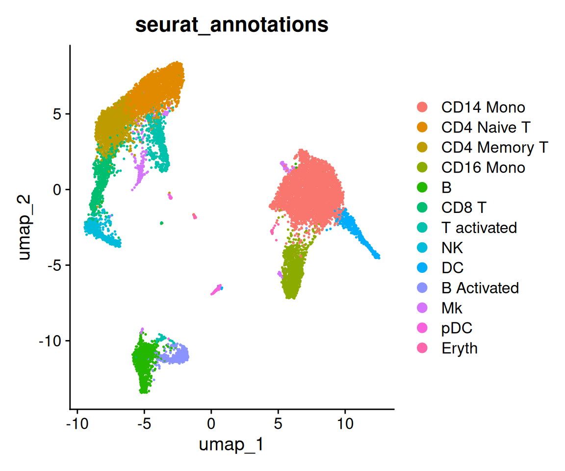
For this example, a cell annotation is available

Idents(ifnb)<- "seurat_annotations"
table(Idents(ifnb))

   CD14 Mono  CD4 Naive T CD4 Memory T    CD16 Mono            B        CD8 T 
        4362         2504         1762         1044          978          814 
 T activated           NK           DC  B Activated           Mk          pDC 
         633          619          472          388          236          132 
       Eryth 
          55 

Differential analysis

Warnings

• The term “differential analysis” is vague/large
• It is important to well formulate the question and know the data design

(a) Das, Rai, and Rai (2022)

(b) Nguyen et al. (2023)

Figure 1: Differential analysis methods

Q: Identify conserved cell type markers

• Goal: identify canonical cell type marker genes that are conserved across conditions

• In function FindConservedMarkers(): DE gene testing for each condition + combine pvalues, based on a function of MetaDE R package (by default, Tippett’s method). For more details on the methods available in metap package, see here.

Example for the cluster of NK cells

Idents(ifnb) <- "seurat_annotations"
NK.markers <- FindConservedMarkers(ifnb, 
                                   ident.1 = "NK", 
                                   grouping.var = "stim", 
                                   verbose = FALSE)
head(NK.markers)

      CTRL_p_val CTRL_avg_log2FC CTRL_pct.1 CTRL_pct.2 CTRL_p_val_adj
GNLY           0        6.854586      0.943      0.046              0
NKG7           0        5.358881      0.953      0.085              0
GZMB           0        5.078135      0.839      0.044              0
CLIC3          0        5.765314      0.601      0.024              0
CTSW           0        5.307246      0.537      0.030              0
KLRD1          0        5.261553      0.507      0.019              0
      STIM_p_val STIM_avg_log2FC STIM_pct.1 STIM_pct.2 STIM_p_val_adj max_pval
GNLY           0        6.435910      0.956      0.059              0        0
NKG7           0        4.971397      0.950      0.081              0        0
GZMB           0        5.151924      0.897      0.060              0        0
CLIC3          0        5.505208      0.623      0.031              0        0
CTSW           0        5.240729      0.592      0.035              0        0
KLRD1          0        4.852457      0.555      0.027              0        0
      minimump_p_val
GNLY               0
NKG7               0
GZMB               0
CLIC3              0
CTSW               0
KLRD1              0

Q: DE genes between two conditions

• Goal: identify genes whose expression varies between the two conditions (cell types combined)

• Design in the example ifnb (see exercice):

  • two conditions: STIM vs CTRL
  • add the sample IDs of each cell

table(ifnb$donor_id)

 SNG-101 SNG-1015 SNG-1016 SNG-1039  SNG-107 SNG-1244 SNG-1256 SNG-1488 
    1197     3116     1438      663      652     1998     2363     2241 

Wilcoxon test (Naive method)

Idents(ifnb)<-ifnb$stim
res1_Wilcox <- FindMarkers(object = ifnb, 
                           ident.1 = "STIM", 
                           ident.2 = "CTRL",
                           test.use = "wilcox")

Percent of genes with adjusted p-value \(<0.01\): 34.67 \(\%\)

genetop_wilcox1<-res1_Wilcox %>%
   filter(p_val_adj<0.01)%>%
   arrange(desc(abs(avg_log2FC)))%>%
   top_n(100)

DESeq2 (Love, Huber, and Anders 2014) - pseudo-bulk method

• From single-cell data to pseudo-bulk data: function AggregateExpression()

pseudo_ifnb1 <- AggregateExpression(ifnb, 
                                   assays = "RNA", 
                                   return.seurat = T, 
                                   group.by = c("stim", "donor_id"))

head(pseudo_ifnb1)

                 orig.ident stim donor_id
CTRL_SNG-101   CTRL_SNG-101 CTRL  SNG-101
CTRL_SNG-1015 CTRL_SNG-1015 CTRL SNG-1015
CTRL_SNG-1016 CTRL_SNG-1016 CTRL SNG-1016
CTRL_SNG-1039 CTRL_SNG-1039 CTRL SNG-1039
CTRL_SNG-107   CTRL_SNG-107 CTRL  SNG-107
CTRL_SNG-1244 CTRL_SNG-1244 CTRL SNG-1244
CTRL_SNG-1256 CTRL_SNG-1256 CTRL SNG-1256
CTRL_SNG-1488 CTRL_SNG-1488 CTRL SNG-1488
STIM_SNG-101   STIM_SNG-101 STIM  SNG-101
STIM_SNG-1015 STIM_SNG-1015 STIM SNG-1015

• Using DESeq2 with Seurat object
• Using DESeq2 on pseudo-bulk data
• Results

Idents(pseudo_ifnb1)<-"stim"
bulk.cond1 <- FindMarkers(object = pseudo_ifnb1, 
                         ident.1 = "STIM", 
                         ident.2 = "CTRL",
                         test.use = "DESeq2")

Percent of genes with adjusted p-value \(<0.01\): 7.42 \(\%\)

library(DESeq2)
cts1<-as.matrix(pseudo_ifnb1@assays$RNA$counts)
coldata1<-pseudo_ifnb1@meta.data
dds1 <- DESeqDataSetFromMatrix(countData = cts1,
                      colData = coldata1,
                      design= ~ donor_id + stim) 
dds1 <- DESeq(dds1,fitType = c("local"))                      
resDEseq1<-results(dds1,name="stim_STIM_vs_CTRL")

Percent of genes with adjusted p-value\(<0.01\): 17.47 \(\%\)

genetopDEseq1<-as.data.frame(resDEseq1) %>%
   filter(padj<0.01)%>%
   arrange(desc(abs(log2FoldChange)))%>%
   top_n(200)

NEBULA (specific single-cell method)

• NEBULA = NEgative Binomial mixed model Using a Large-sample Approximation (He et al. 2021)

library(nebula)
ifnb_neb1<-scToNeb(obj=ifnb,assay="RNA",id="donor_id",pred=c("stim","seurat_annotations"))
df1 = model.matrix(~stim+seurat_annotations, data=ifnb_neb1$pred)
data_g = group_cell(count=ifnb_neb1$count,id=ifnb_neb1$id,pred=df1) 
re1 = nebula(data_g$count,data_g$id,pred=data_g$pred)

Percent of genes with adjusted p-value: \(<0.01\): \(49.1\%\)

Comparison

library(ggvenn)
ggvenn(list(DEseq2=rownames(genetopDEseq1),
            Nebula=genetopNeb1$gene,
            Wilcox=rownames(genetop_wilcox1)))

Q: DE genes between two conditions for “CD14 Mono” cells

• We only consider the cellular type “CD14 Mono”
• Goal: identify genes whose expression varies between the two conditions for the fixed cellular type “CD14 Mono”
• We compare Wilcoxon, DESeq2 and NEBULA

Q: DE genes between two conditions for “CD14 Mono” cells

Comparison

Result with DESeq2

Gene selection via Random Forest

library(randomForest)
datatrain<-t(as.matrix(ifnb@assays$RNA$scale.data[,ICD14Mono]))
dataRF<-data.frame(datatrain,
                   Cl = as.factor(ifnb$stim[ICD14Mono]))
resRF<-randomForest(Cl ~ ., data = dataRF,importance=T,proximity=T)

Gene selection via Random Forest

Gene functional analysis

Gene enrichment analysis identifies biological pathways or functions that are overrepresented in a set of genes of interest.

In functional analysis of biological pathway, the biologist is always the expert :

• The pathway database is determinent.
• You decide the relationship and biological significance of the data you want to present.

Why ?

The interpretation of the list of differentially expressed genes can be challenging due to two scenarios:

1. The list is so long that it becomes cumbersome and time-consuming to analyze and interpret each gene individually.
2. Some genes may have low p-values but not low enough to meet the given threshold for significance.

In such situations, enrichment analysis can be employed to enhance the understanding of our dataset.

Approaches

1. Over Representation Analysis (ORA): This method determines whether the differentially expressed genes are enriched in specific pathways or ontological groups.
2. Gene Set Enrichment Analysis (GSEA): GSEA evaluates whether a pre-defined set of genes (gene set) shows statistically significant differences between two or more biological conditions.

Various sources of biological pathways

1. Gene Ontology (GO)
2. KEGG (Kyoto Encyclopedia of Genes and Genomes)
3. WikiPathways
4. Disease Ontology
5. Reactome
6. MSigDB (Molecular Signatures Database)
7. MeSH (Medical Subject Headings)

From (Gene) Symbols to (Gene) IDs

Gene identifiers are unique, stable, and standardized, unlike gene symbols, which are often ambiguous.

They allow for:

• Reliable annotation through databases like Ensembl
  
• Cross-species comparisons
  
• Data integration across studies
  
• Reproducibility and long-term accessibility

bitr: Biological Id TranslatoR

require(clusterProfiler)
genes <- bulk.cond1  |> filter(p_val_adj<0.01)  |> rownames()
eg = bitr(genes, fromType="SYMBOL", toType="ENTREZID", OrgDb="org.Hs.eg.db")

Gene Ontology (GO)

Site web : http://geneontology.org/

Description :

GO is a widely used database that categorizes genes into three main ontologies:

1. Molecular Function
   • Describes the elemental activities of a gene product at the molecular level.
2. Biological Process
   • Represents sets of molecular events or biological pathways achieved by one or more gene products.
   • Biological process terms describe the larger, coordinated series of events that involve multiple molecular functions.
3. Cellular Component
   • Refers to the subcellular structures, locations, and macromolecular complexes in which gene products are active.
   • Cellular component terms describe the physical compartments or structures where gene products function.

Tip

• Ten Quick Tips for Using the Gene Ontology

Over Representation analysis

Over Representation Analysis (ORA) is a widely used approach to determine whether known biological functions or processes are over-represented (= enriched) in an experimentally-derived gene list, e.g. a list of differentially expressed genes (DEGs).

From bioinformatics-core-shared-training.github.io/Bulk_RNAseq_Course_Apr22

GO over-representation analysis with R

The clusterProfiler package implements enrichGO() for gene ontology over-representation test.

org.db <- org.Hs.eg.db::org.Hs.eg.db
ego <- enrichGO(gene          = eg$ENTREZID,
                universe      = NULL,
                OrgDb         = org.db,
                keyType = "ENTREZID",
                ont           = "BP",
                pAdjustMethod = "BH",
                pvalueCutoff  = 0.05,
                qvalueCutoff  = 0.05,
                readable      = TRUE)

ego |> as_tibble() |>  rmarkdown::paged_table()

Some extensions/complements

Spatial transcriptomic (ST)

ST Data

• The spot by gene expression matrix

• The information necessary to associate spots with their physical position on the tissue image

Spatial transcriptomic (ST)

Example

• Mouse brain spatial expression for the anterior region (\(G=31053\) genes across \(C=2696\) spots)

#InstallData("stxBrain")
brain <- LoadData("stxBrain", type = "anterior1")
brain

An object of class Seurat 
31053 features across 2696 samples within 1 assay 
Active assay: Spatial (31053 features, 0 variable features)
 1 layer present: counts
 1 spatial field of view present: anterior1

SpatialFeaturePlot(brain, features = "nCount_Spatial") + 
  theme(legend.position = "right")

brain@assays$Spatial$counts[1:6,1:10]

6 x 10 sparse Matrix of class "dgCMatrix"

                           
Xkr4    . . . . . . . . . .
Gm1992  . . . . . . . . . .
Gm37381 . . . . . . . . . .
Rp1     . . . . . . . . . .
Sox17   . 1 . . . 2 . . 1 .
Gm37323 . . . . . . . . . .

brain@images$anterior1

Spatial coordinates for 2696 cells
Default segmentation boundary: centroids 
Associated assay: Spatial 
Key: slice1_ 

Analysis Pipeline of ST data

Pipeline

• Normalization
• Dimension reduction
• Clustering : take into account spatial information
• Marker genes
• ….
• Detecting spatially-variable features

Spatial transcriptomic (ST)

Normalization

• Variance in molecular counts across spots is not just technical in nature, but also is dependent on the tissue anatomy
• Standard approaches (such as the LogNormalize() function), which force each data point to have the same underlying “size” after normalization, can be problematic
• Recommend using sctransform (Hafemeister and Satija 2019a)
• SCTransform() replaces NormalizeData(), ScaleData(), and FindVariableFeatures()

• SCTransform
• VariableFeaturePlot
• SpatialFeaturePlot

brain <- SCTransform(brain, 
            assay = "Spatial",
            verbose = FALSE)
brain@assays$SCT

SCTAssay data with 17668 features for 2696 cells, and 1 SCTModel(s) 
Top 10 variable features:
 Ttr, Hbb-bs, Mbp, Plp1, Hba-a1, Ptgds, Penk, S100a5, Hba-a2, Fabp7 

VariableFeaturePlot(brain)

SpatialFeaturePlot(brain, features = c("Ttr","Hbb-bs"))

Spatial transcriptomic (ST)

Dimension reduction

Spatial transcriptomic (ST)

Clustering

• Some clustering methods for ST

(Cheng, Hu, and Li 2023)

(Xiong et al. 2025)

Example with BayesSpace

Caution

See code in exercice !

Spatial variable features

• Goal: Identify features whose variability in expression can be explained to some degree by spatial location

Seurat

• Function FindSpatiallyVariableFeatures()

• Methods:

  • markvariogram: Wraps the functionality of markvario from the spatstat package (Wälder and Stoyan 1996)
  • moransi: Wraps the functionality of the Moran.I function from the ape package (Gittleman and Kot 1990)

• Other approaches in the literature: SpatialDE and Splotch for instance

brain <- FindSpatiallyVariableFeatures(brain, 
                                       assay = "SCT", 
                                       features=VariableFeatures(brain)[1:1000],
                                       selection.method = "moransi")

Pseudotime

Principle of trajectory inference

• Trajectory inference aims to reconstruct a cellular dynamic process
• 2 main steps:
  • Dimensionality reduction step: PCA, t-SNE, . . . . or graph-based techniques . . . . or clustering methods
  • Trajectory modelling step

Pseudotime

Review

• Some references:
  • (Cannoodt, Saelens, and Saeys 2016) : comparison of 10 methods
  • (Saelens et al. 2019) : comparison of 29 (among 59 existing) methods
  • Dyno contains a set of package to infer, visualise and interpret single-cell trajectories

AnnData

Schematic representation of the AnnData object

• X: Count data in sparse matrix format:

  • adata.X
    <100x2000 sparse matrix of type '<class 'numpy.float32'>'
      with 126526 stored elements in Compressed Sparse Row format>

  • adata.obs_names = [f"Cell_{i:d}" for i in range(adata.n_obs)]
    adata.var_names = [f"Gene_{i:d}" for i in range(adata.n_vars)]
    print(adata.obs_names[:10])
    Index(['Cell_0', 'Cell_1', 'Cell_2', 'Cell_3', 'Cell_4', 'Cell_5', 'Cell_6',
         'Cell_7', 'Cell_8', 'Cell_9'],
        dtype='object')

• obs/var: Metadata for observations and variables
  
• Layers: adata.layers["log_transformed"] = np.log1p(adata.X)
  
• obsm/varm: Additional derived metrics or data related to observations / variables (e.g., PCA results)
  
• uns: Unstructured data (analysis parameters, other metadata, etc.)
  
• obsp/varp: Pairwise relationships between cells
  

How to switch between Seurat / Scanpy / SingleCellExperiment

• SeuratDisk: the solution provided by Seurat to convert to various format \(\rightarrow\) not working
• anndata2ri: a python package developped to convert AnnData\(\Leftrightarrow\)SingleCellExperiment
• zellkonverter: a R package developped to convert SingleCellExperiment\(\rightarrow\) various objects.
• Seurat\(\rightarrow\)AnnData can be done by hand \(\rightarrow\) details here

Within R

sce_ifnb <- as.SingleCellExperiment(ifnb)

library(zellkonverter)
library(reticulate)
writeH5AD(sce_ifnb, file = "sce_ifnb.h5ad")

Within python

import anndata as ad
adata = ad.read('sce_ifnb.h5ad', backed='r')
adata
AnnData object with n_obs × n_vars = 13668 × 14053 backed at 'conversion_files/sce_ifnb.h5ad'
    obs: 'orig.ident', 'nCount_RNA', 'nFeature_RNA', 'stim', 'seurat_annotations', 'RNA_snn_res.0.5', 'seurat_clusters', 'donor_id', 'celltype.stim', 'ident'
    uns: 'X_name'
    obsm: 'INTEGRATED.CCA', 'PCA', 'UMAP', 'UMAP.UNINTEGRATED'
    layers: 'logcounts'

I want to stay in R

Stay in R:

adata <- SCE2AnnData(sce_ifnb)
adata

References

Baysoy, Alev, Zhiliang Bai, Rahul Satija, and Rong Fan. 2023. “The Technological Landscape and Applications of Single-Cell Multi-Omics.” Nature Reviews Molecular Cell Biology 24 (10): 695–713.

Becht, Etienne, Leland McInnes, John Healy, Charles-Antoine Dutertre, Immanuel WH Kwok, Lai Guan Ng, Florent Ginhoux, and Evan W Newell. 2019. “Dimensionality Reduction for Visualizing Single-Cell Data Using UMAP.” Nature Biotechnology 37 (1): 38–44.

Butler, Andrew, Paul Hoffman, Peter Smibert, Efthymia Papalexi, and Rahul Satija. 2018. “Integrating Single-Cell Transcriptomic Data Across Different Conditions, Technologies, and Species.” Nature Biotechnology 36: 411–20. https://doi.org/10.1038/nbt.4096.

Cannoodt, Robrecht, Wouter Saelens, and Yvan Saeys. 2016. “Computational Methods for Trajectory Inference from Single-Cell Transcriptomics.” European Journal of Immunology 46 (11): 2496–506.

Cheng, Andrew, Guanyu Hu, and Wei Vivian Li. 2023. “Benchmarking Cell-Type Clustering Methods for Spatially Resolved Transcriptomics Data.” Briefings in Bioinformatics 24 (1): bbac475.

Das, Samarendra, Anil Rai, and Shesh N Rai. 2022. “Differential Expression Analysis of Single-Cell RNA-Seq Data: Current Statistical Approaches and Outstanding Challenges.” Entropy 24 (7): 995.

Gittleman, John L, and Mark Kot. 1990. “Adaptation: Statistics and a Null Model for Estimating Phylogenetic Effects.” Systematic Zoology 39 (3): 227–41.

Guo, Minzhe, Hui Wang, S Steven Potter, Jeffrey A Whitsett, and Yan Xu. 2015. “SINCERA: A Pipeline for SINgle-CEll RNA-seq Profiling Analysis.” PLoS Comput. Biol. 11 (11): e1004575.

Hafemeister, Christoph, and Rahul Satija. 2019a. “Normalization and Variance Stabilization of Single-Cell RNA-Seq Data Using Regularized Negative Binomial Regression.” Genome Biology 20 (1): 296.

———. 2019b. “Normalization and Variance Stabilization of Single-Cell RNA-seq Data Using Regularized Negative Binomial Regression.” Genome Biol. 20 (1): 296.

Hao, Yuhan, Stephanie Hao, Erica Andersen-Nissen, William M. Mauck III, Shiwei Zheng, Andrew Butler, Maddie J. Lee, et al. 2021. “Integrated Analysis of Multimodal Single-Cell Data.” Cell. https://doi.org/10.1016/j.cell.2021.04.048.

Hao, Yuhan, Tim Stuart, Madeline H Kowalski, Saket Choudhary, Paul Hoffman, Austin Hartman, Avi Srivastava, et al. 2023. “Dictionary Learning for Integrative, Multimodal and Scalable Single-Cell Analysis.” Nature Biotechnology. https://doi.org/10.1038/s41587-023-01767-y.

He, Liang, Jose Davila-Velderrain, Tomokazu S Sumida, David A Hafler, Manolis Kellis, and Alexander M Kulminski. 2021. “NEBULA Is a Fast Negative Binomial Mixed Model for Differential or Co-Expression Analysis of Large-Scale Multi-Subject Single-Cell Data.” Communications Biology 4 (1): 629.

Juliá, Miguel, Amalio Telenti, and Antonio Rausell. 2015. “Sincell: An R/Bioconductor Package for Statistical Assessment of Cell-State Hierarchies from Single-Cell RNA-seq.” Bioinformatics 31 (20): 3380–82.

Korsunsky, Ilya, Nghia Millard, Jean Fan, Kamil Slowikowski, Fan Zhang, Kevin Wei, Yuriy Baglaenko, Michael Brenner, Po-ru Loh, and Soumya Raychaudhuri. 2019. “Fast, Sensitive and Accurate Integration of Single-Cell Data with Harmony.” Nature Methods 16 (12): 1289–96.

Love, Michael I, Wolfgang Huber, and Simon Anders. 2014. “Moderated Estimation of Fold Change and Dispersion for RNA-Seq Data with DESeq2.” Genome Biology 15: 1–21.

Lun, Aaron T L, Davis J McCarthy, and John C Marioni. 2016. “A Step-by-Step Workflow for Low-Level Analysis of Single-Cell RNA-seq Data with Bioconductor.” F1000Res. 5 (August): 2122.

Maaten, Laurens van der, and Geoffrey Hinton. 2008. “Visualizing Data Using t-SNE.” Journal of Machine Learning Research 9 (Nov): 2579–2605.

McInnes, Leland, John Healy, and James Melville. 2018. “Umap: Uniform Manifold Approximation and Projection for Dimension Reduction.” arXiv Preprint arXiv:1802.03426.

Nguyen, Hai CT, Bukyung Baik, Sora Yoon, Taesung Park, and Dougu Nam. 2023. “Benchmarking Integration of Single-Cell Differential Expression.” Nature Communications 14 (1): 1570.

Rostom, Raghd, Valentine Svensson, Sarah A Teichmann, and Gozde Kar. 2017. “Computational Approaches for Interpreting Sc RNA-Seq Data.” FEBS Letters 591 (15): 2213–25.

Saelens, Wouter, Robrecht Cannoodt, Helena Todorov, and Yvan Saeys. 2019. “A Comparison of Single-Cell Trajectory Inference Methods.” Nature Biotechnology 37 (5): 547–54.

Satija, Rahul, Jeffrey A Farrell, David Gennert, Alexander F Schier, and Aviv Regev. 2015. “Spatial Reconstruction of Single-Cell Gene Expression Data.” Nature Biotechnology 33: 495–502. https://doi.org/10.1038/nbt.3192.

Specque, Florian, Aurélien Barré, Macha Nikolski, and Domitille Chalopin. 2024. “SeuratIntegrate: An R Package to Facilitate the Use of Integration Methods with Seurat.” bioRxiv.

Stuart, Tim, Andrew Butler, Paul Hoffman, Christoph Hafemeister, Efthymia Papalexi, William M Mauck III, Yuhan Hao, Marlon Stoeckius, Peter Smibert, and Rahul Satija. 2019. “Comprehensive Integration of Single-Cell Data.” Cell 177: 1888–1902. https://doi.org/10.1016/j.cell.2019.05.031.

Van Der Maaten, Laurens. 2014. “Accelerating t-SNE Using Tree-Based Algorithms.” The Journal of Machine Learning Research 15 (1): 3221–45.

Wälder, Olga, and Dietrich Stoyan. 1996. “On Variograms in Point Process Statistics.” Biometrical Journal 38 (8): 895–905.

Wolf, F Alexander, Philipp Angerer, and Fabian J Theis. 2018. “SCANPY: Large-Scale Single-Cell Gene Expression Data Analysis.” Genome Biol. 19 (1).

Xiong, Caiwei, Huang Shuai, Muqing Zhou, Yiyan Zhang, Wenrong Wu, Xihao Li, Huaxiu Yao, Jiawen Chen, and Yun Li. 2025. “A Comprehensive Comparison on Clustering Methods for Multi-Slide Spatially Resolved Transcriptomics Data Analysis.” bioRxiv, 2025–01.

Zhang, Yuanchao, Man S Kim, Erin R Reichenberger, Ben Stear, and Deanne M Taylor. 2020. “Scedar: A Scalable Python Package for Single-Cell RNA-seq Exploratory Data Analysis.” PLoS Comput. Biol. 16 (4): e1007794.